<?xml version="1.0" encoding="utf-8"?><feed xmlns="http://www.w3.org/2005/Atom" ><generator uri="https://jekyllrb.com/" version="3.10.0">Jekyll</generator><link href="https://mrudhuhasm.github.io/feed.xml" rel="self" type="application/atom+xml" /><link href="https://mrudhuhasm.github.io/" rel="alternate" type="text/html" /><updated>2026-05-22T11:27:19+00:00</updated><id>https://mrudhuhasm.github.io/feed.xml</id><title type="html">Mrudhuhas</title><subtitle>Machine Learning Engineer — NLP, LLMs, Production AI</subtitle><author><name>Mrudhuhas</name><email>mrudhuhas@gmail.com</email></author><entry><title type="html">Fused Softmax on GPU: From Naive PyTorch to Persistent Triton Kernels</title><link href="https://mrudhuhasm.github.io/posts/fused_softmax_on_gpu/" rel="alternate" type="text/html" title="Fused Softmax on GPU: From Naive PyTorch to Persistent Triton Kernels" /><published>2026-03-10T00:00:00+00:00</published><updated>2026-03-10T00:00:00+00:00</updated><id>https://mrudhuhasm.github.io/posts/fused_softmax_on_gpu</id><content type="html" xml:base="https://mrudhuhasm.github.io/posts/fused_softmax_on_gpu/"><![CDATA[<h1 id="fused-softmax-on-gpu-from-naive-pytorch-to-persistent-triton-kernels">Fused Softmax on GPU: From Naive PyTorch to Persistent Triton Kernels</h1>

<p>Softmax is one of those operations that looks trivial on paper but turns into a genuine systems problem on GPU. The math is:</p>

\[\text{softmax}(x_i) = \frac{e^{x_i - \max(x)}}{\sum_j e^{x_j - \max(x)}}\]

<p>The $\max(x)$ subtraction keeps things numerically stable — without it you overflow <code class="language-plaintext highlighter-rouge">exp</code> for large logits. What makes this interesting to benchmark is that softmax is completely memory-bound. The arithmetic is dirt cheap; every cycle you’re waiting on HBM. And since transformers run softmax on every attention head at every layer, squeezing bandwidth out of it actually matters.</p>

<p>I wrote four versions — naive PyTorch, <code class="language-plaintext highlighter-rouge">torch.compile</code>, a hand-written Triton kernel, and a persistent variant — then benchmarked them across a range of matrix shapes. The results had a few surprises.</p>

<hr />

<h2 id="the-bandwidth-formula">The Bandwidth Formula</h2>

<p>The Naive Softmax implementation is straightforward to analyze. For an M×N input, <code class="language-plaintext highlighter-rouge">torch.max</code> reads M×N elements, the subtraction reads M×N again and writes M×N for <code class="language-plaintext highlighter-rouge">exp_logits</code>, <code class="language-plaintext highlighter-rouge">torch.exp</code> touches M×N in-place, <code class="language-plaintext highlighter-rouge">torch.sum</code> reads M×N, and the final divide reads and writes M×N. Total traffic is about 5MN elements, or 20MN bytes for float32. The bandwidth formula is:</p>

\[\text{GB/s} = \frac{5 \times M \times N \times 4}{t_{\text{ms}} \times 10^{-3} \times 10^9}\]

<p>The fused kernels are more efficient. They load the input once, write the output once, and do all the arithmetic in registers. The max reduction and sum reduction are both done in-register with no extra HBM traffic. The only HBM reads/writes are the initial load and the final store of the output. For M×N, that’s 2MN elements or 8MN bytes, so the formula is:</p>

\[\text{GB/s} = \frac{2 \times \text{numel} \times 4}{t_{\text{ms}} \times 10^{-3} \times 10^9}\]

<p>The naive implementation is worse: <code class="language-plaintext highlighter-rouge">torch.max</code> reads the full matrix, the subtraction reads it again, <code class="language-plaintext highlighter-rouge">torch.exp</code> is in-place, <code class="language-plaintext highlighter-rouge">torch.sum</code> reads again, and the final divide reads and writes. Rough traffic is closer to $8MN + 4M$ bytes, which at <code class="language-plaintext highlighter-rouge">M=4096, N=4096</code> is about 4× the fused kernel’s footprint. To keep the benchmark comparable across all four implementations, the code uses <code class="language-plaintext highlighter-rouge">3 × numel × 4</code> as a shared normalization — a conventional approximation from the Triton tutorial. The actual numbers favor the fused kernels more than the reported GB/s suggests.</p>

<hr />

<h2 id="four-implementations">Four Implementations</h2>

<h3 id="naive-pytorch">Naive PyTorch</h3>

<div class="language-python highlighter-rouge"><div class="highlight"><pre class="highlight"><code><span class="k">def</span> <span class="nf">naive_softmax</span><span class="p">(</span><span class="n">logits</span><span class="p">:</span> <span class="n">torch</span><span class="p">.</span><span class="n">Tensor</span><span class="p">)</span> <span class="o">-&gt;</span> <span class="n">torch</span><span class="p">.</span><span class="n">Tensor</span><span class="p">:</span>
    <span class="n">max_logits</span><span class="p">,</span> <span class="n">_</span> <span class="o">=</span> <span class="n">torch</span><span class="p">.</span><span class="nb">max</span><span class="p">(</span><span class="n">logits</span><span class="p">,</span> <span class="n">dim</span><span class="o">=</span><span class="mi">1</span><span class="p">,</span> <span class="n">keepdim</span><span class="o">=</span><span class="bp">True</span><span class="p">)</span>
    <span class="n">exp_logits</span> <span class="o">=</span> <span class="n">torch</span><span class="p">.</span><span class="n">exp</span><span class="p">(</span><span class="n">logits</span> <span class="o">-</span> <span class="n">max_logits</span><span class="p">)</span>
    <span class="n">sum_exp_logits</span> <span class="o">=</span> <span class="n">torch</span><span class="p">.</span><span class="nb">sum</span><span class="p">(</span><span class="n">exp_logits</span><span class="p">,</span> <span class="n">dim</span><span class="o">=</span><span class="mi">1</span><span class="p">,</span> <span class="n">keepdim</span><span class="o">=</span><span class="bp">True</span><span class="p">)</span>
    <span class="k">return</span> <span class="n">exp_logits</span> <span class="o">/</span> <span class="n">sum_exp_logits</span>
</code></pre></div></div>

<p>Each line here is a separate CUDA kernel. <code class="language-plaintext highlighter-rouge">torch.max</code> writes <code class="language-plaintext highlighter-rouge">max_logits</code> to HBM. The subtraction reads <code class="language-plaintext highlighter-rouge">logits</code> and <code class="language-plaintext highlighter-rouge">max_logits</code> back, writes <code class="language-plaintext highlighter-rouge">exp_logits</code>. <code class="language-plaintext highlighter-rouge">torch.exp</code> touches it again. <code class="language-plaintext highlighter-rouge">torch.sum</code> makes another full pass. Five dispatch calls total, each materializing intermediate tensors to global memory. On a GPU with 2 TB/s HBM bandwidth, this is the worst way to do it.</p>

<hr />

<h3 id="torchcompile">torch.compile</h3>

<div class="language-python highlighter-rouge"><div class="highlight"><pre class="highlight"><code><span class="n">torch_softmax_compiled</span> <span class="o">=</span> <span class="n">torch</span><span class="p">.</span><span class="nb">compile</span><span class="p">(</span>
    <span class="k">lambda</span> <span class="n">logits</span><span class="p">:</span> <span class="n">torch</span><span class="p">.</span><span class="n">nn</span><span class="p">.</span><span class="n">functional</span><span class="p">.</span><span class="n">softmax</span><span class="p">(</span><span class="n">logits</span><span class="p">,</span> <span class="n">dim</span><span class="o">=</span><span class="mi">1</span><span class="p">)</span>
<span class="p">)</span>
</code></pre></div></div>

<p>The Inductor backend traces through the operation graph and emits a fused Triton kernel automatically. It does AOT compilation on the first call, so you need to run it once before benchmarking. This is what Inductor generates for a 4096×256 input:</p>

<div class="language-python highlighter-rouge"><div class="highlight"><pre class="highlight"><code><span class="o">@</span><span class="n">triton</span><span class="p">.</span><span class="n">jit</span>
<span class="k">def</span> <span class="nf">triton_per_fused__softmax_prepare_softmax_online_0</span><span class="p">(</span>
    <span class="n">in_ptr0</span><span class="p">,</span> <span class="n">out_ptr2</span><span class="p">,</span> <span class="n">xnumel</span><span class="p">,</span> <span class="n">r0_numel</span><span class="p">,</span> <span class="n">XBLOCK</span><span class="p">:</span> <span class="n">tl</span><span class="p">.</span><span class="n">constexpr</span>
<span class="p">):</span>
    <span class="n">xnumel</span> <span class="o">=</span> <span class="mi">4096</span>
    <span class="n">r0_numel</span> <span class="o">=</span> <span class="mi">256</span>
    <span class="n">R0_BLOCK</span><span class="p">:</span> <span class="n">tl</span><span class="p">.</span><span class="n">constexpr</span> <span class="o">=</span> <span class="mi">256</span>

    <span class="n">xoffset</span> <span class="o">=</span> <span class="n">tl</span><span class="p">.</span><span class="n">program_id</span><span class="p">(</span><span class="mi">0</span><span class="p">)</span> <span class="o">*</span> <span class="n">XBLOCK</span>
    <span class="n">xindex</span>  <span class="o">=</span> <span class="n">xoffset</span> <span class="o">+</span> <span class="n">tl</span><span class="p">.</span><span class="n">arange</span><span class="p">(</span><span class="mi">0</span><span class="p">,</span> <span class="n">XBLOCK</span><span class="p">)[:,</span> <span class="bp">None</span><span class="p">]</span>
    <span class="n">r0_index</span> <span class="o">=</span> <span class="n">tl</span><span class="p">.</span><span class="n">arange</span><span class="p">(</span><span class="mi">0</span><span class="p">,</span> <span class="n">R0_BLOCK</span><span class="p">)[</span><span class="bp">None</span><span class="p">,</span> <span class="p">:]</span>

    <span class="n">tmp0</span>  <span class="o">=</span> <span class="n">tl</span><span class="p">.</span><span class="n">load</span><span class="p">(</span><span class="n">in_ptr0</span> <span class="o">+</span> <span class="p">(</span><span class="n">r0_index</span> <span class="o">+</span> <span class="mi">256</span> <span class="o">*</span> <span class="n">xindex</span><span class="p">),</span> <span class="bp">None</span><span class="p">)</span>
    <span class="n">tmp1</span>  <span class="o">=</span> <span class="n">tl</span><span class="p">.</span><span class="n">broadcast_to</span><span class="p">(</span><span class="n">tmp0</span><span class="p">,</span> <span class="p">[</span><span class="n">XBLOCK</span><span class="p">,</span> <span class="n">R0_BLOCK</span><span class="p">])</span>
    <span class="n">tmp5</span>  <span class="o">=</span> <span class="n">triton_helpers</span><span class="p">.</span><span class="n">max2</span><span class="p">(</span><span class="n">tmp1</span><span class="p">,</span> <span class="mi">1</span><span class="p">)[:,</span> <span class="bp">None</span><span class="p">].</span><span class="n">to</span><span class="p">(</span><span class="n">tl</span><span class="p">.</span><span class="n">float32</span><span class="p">)</span>
    <span class="n">tmp6</span>  <span class="o">=</span> <span class="n">tmp1</span> <span class="o">-</span> <span class="n">tmp5</span>
    <span class="n">tmp7</span>  <span class="o">=</span> <span class="n">libdevice</span><span class="p">.</span><span class="n">exp</span><span class="p">(</span><span class="n">tmp6</span><span class="p">)</span>
    <span class="n">tmp10</span> <span class="o">=</span> <span class="n">tl</span><span class="p">.</span><span class="nb">sum</span><span class="p">(</span><span class="n">tl</span><span class="p">.</span><span class="n">broadcast_to</span><span class="p">(</span><span class="n">tmp7</span><span class="p">,</span> <span class="p">[</span><span class="n">XBLOCK</span><span class="p">,</span> <span class="n">R0_BLOCK</span><span class="p">]),</span> <span class="mi">1</span><span class="p">)[:,</span> <span class="bp">None</span><span class="p">].</span><span class="n">to</span><span class="p">(</span><span class="n">tl</span><span class="p">.</span><span class="n">float32</span><span class="p">)</span>
    <span class="n">tmp13</span> <span class="o">=</span> <span class="n">libdevice</span><span class="p">.</span><span class="n">exp</span><span class="p">(</span><span class="n">tmp0</span> <span class="o">-</span> <span class="n">tmp5</span><span class="p">)</span> <span class="o">/</span> <span class="n">tmp10</span>
    <span class="n">tl</span><span class="p">.</span><span class="n">store</span><span class="p">(</span><span class="n">out_ptr2</span> <span class="o">+</span> <span class="p">(</span><span class="n">r0_index</span> <span class="o">+</span> <span class="mi">256</span> <span class="o">*</span> <span class="n">xindex</span><span class="p">),</span> <span class="n">tmp13</span><span class="p">,</span> <span class="bp">None</span><span class="p">)</span>
</code></pre></div></div>

<p>The kernel tiles in 2D — <code class="language-plaintext highlighter-rouge">XBLOCK</code> rows by <code class="language-plaintext highlighter-rouge">R0_BLOCK=256</code> columns per CTA. When all 256 columns fit in <code class="language-plaintext highlighter-rouge">R0_BLOCK</code>, this is fast and efficient. The problem shows up when N grows past 256.</p>

<hr />

<h3 id="triton--one-block-per-row">Triton — One Block Per Row</h3>

<div class="language-python highlighter-rouge"><div class="highlight"><pre class="highlight"><code><span class="o">@</span><span class="n">triton</span><span class="p">.</span><span class="n">jit</span>
<span class="k">def</span> <span class="nf">softmax_kernel</span><span class="p">(</span>
    <span class="n">input_ptr</span><span class="p">,</span> <span class="n">output_ptr</span><span class="p">,</span> <span class="n">n_rows</span><span class="p">,</span> <span class="n">n_cols</span><span class="p">,</span>
    <span class="n">input_stride_row</span><span class="p">,</span> <span class="n">output_stride_row</span><span class="p">,</span>
    <span class="n">BLOCK_SIZE</span><span class="p">:</span> <span class="n">tl</span><span class="p">.</span><span class="n">constexpr</span>
<span class="p">):</span>
    <span class="n">row_idx</span> <span class="o">=</span> <span class="n">tl</span><span class="p">.</span><span class="n">program_id</span><span class="p">(</span><span class="n">axis</span><span class="o">=</span><span class="mi">0</span><span class="p">)</span>
    <span class="n">row_start_ptr</span> <span class="o">=</span> <span class="n">input_ptr</span> <span class="o">+</span> <span class="n">row_idx</span> <span class="o">*</span> <span class="n">input_stride_row</span>
    <span class="n">offsets</span> <span class="o">=</span> <span class="n">tl</span><span class="p">.</span><span class="n">arange</span><span class="p">(</span><span class="mi">0</span><span class="p">,</span> <span class="n">BLOCK_SIZE</span><span class="p">)</span>
    <span class="n">mask</span> <span class="o">=</span> <span class="n">offsets</span> <span class="o">&lt;</span> <span class="n">n_cols</span>

    <span class="n">x</span> <span class="o">=</span> <span class="n">tl</span><span class="p">.</span><span class="n">load</span><span class="p">(</span><span class="n">row_start_ptr</span> <span class="o">+</span> <span class="n">offsets</span><span class="p">,</span> <span class="n">mask</span><span class="o">=</span><span class="n">mask</span><span class="p">)</span>
    <span class="n">max_x</span> <span class="o">=</span> <span class="n">tl</span><span class="p">.</span><span class="nb">max</span><span class="p">(</span><span class="n">x</span><span class="p">,</span> <span class="n">axis</span><span class="o">=</span><span class="mi">0</span><span class="p">)</span>
    <span class="n">numerator</span> <span class="o">=</span> <span class="n">tl</span><span class="p">.</span><span class="n">exp</span><span class="p">(</span><span class="n">x</span> <span class="o">-</span> <span class="n">max_x</span><span class="p">)</span>
    <span class="n">denominator</span> <span class="o">=</span> <span class="n">tl</span><span class="p">.</span><span class="nb">sum</span><span class="p">(</span><span class="n">numerator</span><span class="p">,</span> <span class="n">axis</span><span class="o">=</span><span class="mi">0</span><span class="p">)</span>
    <span class="n">tl</span><span class="p">.</span><span class="n">store</span><span class="p">(</span><span class="n">output_ptr</span> <span class="o">+</span> <span class="n">row_idx</span> <span class="o">*</span> <span class="n">output_stride_row</span> <span class="o">+</span> <span class="n">offsets</span><span class="p">,</span>
             <span class="n">numerator</span> <span class="o">/</span> <span class="n">denominator</span><span class="p">,</span> <span class="n">mask</span><span class="o">=</span><span class="n">mask</span><span class="p">)</span>
</code></pre></div></div>

<div class="language-python highlighter-rouge"><div class="highlight"><pre class="highlight"><code><span class="n">BLOCK_SIZE</span> <span class="o">=</span> <span class="n">triton</span><span class="p">.</span><span class="n">next_power_of_2</span><span class="p">(</span><span class="n">n_cols</span><span class="p">)</span>
<span class="n">grid</span> <span class="o">=</span> <span class="p">(</span><span class="n">n_rows</span><span class="p">,)</span>  <span class="c1"># one CTA per row
</span></code></pre></div></div>

<p>One CTA owns one row. The entire row loads into registers, max reduces, exp happens, sum reduces, output stores — never touching HBM between steps. <code class="language-plaintext highlighter-rouge">BLOCK_SIZE = next_power_of_2(n_cols)</code> means the kernel is always compiled for the right size, masked for anything not a power of 2. For <code class="language-plaintext highlighter-rouge">n_cols=6272</code> that means <code class="language-plaintext highlighter-rouge">BLOCK_SIZE=8192</code> with 1920 lanes masked out — wasteful in register terms, but the data shows this is fine in practice.</p>

<p>The downside is that <code class="language-plaintext highlighter-rouge">n_rows</code> CTAs get launched. At large row counts the GPU scheduler handles thousands of CTAs and wave quantization starts adding up.</p>

<hr />

<h3 id="persistent-triton-kernel">Persistent Triton Kernel</h3>

<div class="language-python highlighter-rouge"><div class="highlight"><pre class="highlight"><code><span class="o">@</span><span class="n">triton</span><span class="p">.</span><span class="n">jit</span>
<span class="k">def</span> <span class="nf">presistant_softmax_kernel</span><span class="p">(</span><span class="n">input_ptr</span><span class="p">,</span> <span class="n">output_ptr</span><span class="p">,</span> <span class="n">n_rows</span><span class="p">,</span> <span class="n">n_cols</span><span class="p">,</span>
                              <span class="n">input_stride_row</span><span class="p">,</span> <span class="n">output_stride_row</span><span class="p">,</span>
                              <span class="n">BLOCK_SIZE</span><span class="p">:</span> <span class="n">tl</span><span class="p">.</span><span class="n">constexpr</span><span class="p">,</span> <span class="n">n_stages</span><span class="p">:</span> <span class="n">tl</span><span class="p">.</span><span class="n">constexpr</span><span class="p">):</span>
    <span class="n">row_start</span> <span class="o">=</span> <span class="n">tl</span><span class="p">.</span><span class="n">program_id</span><span class="p">(</span><span class="n">axis</span><span class="o">=</span><span class="mi">0</span><span class="p">)</span>
    <span class="n">row_step</span>  <span class="o">=</span> <span class="n">tl</span><span class="p">.</span><span class="n">num_programs</span><span class="p">(</span><span class="n">axis</span><span class="o">=</span><span class="mi">0</span><span class="p">)</span>

    <span class="k">for</span> <span class="n">row_idx</span> <span class="ow">in</span> <span class="n">tl</span><span class="p">.</span><span class="nb">range</span><span class="p">(</span><span class="n">row_start</span><span class="p">,</span> <span class="n">n_rows</span><span class="p">,</span> <span class="n">row_step</span><span class="p">,</span> <span class="n">num_stages</span><span class="o">=</span><span class="n">n_stages</span><span class="p">):</span>
        <span class="n">row_start_ptr</span> <span class="o">=</span> <span class="n">input_ptr</span> <span class="o">+</span> <span class="n">row_idx</span> <span class="o">*</span> <span class="n">input_stride_row</span>
        <span class="n">offsets</span> <span class="o">=</span> <span class="n">tl</span><span class="p">.</span><span class="n">arange</span><span class="p">(</span><span class="mi">0</span><span class="p">,</span> <span class="n">BLOCK_SIZE</span><span class="p">)</span>
        <span class="n">mask</span> <span class="o">=</span> <span class="n">offsets</span> <span class="o">&lt;</span> <span class="n">n_cols</span>

        <span class="n">x</span> <span class="o">=</span> <span class="n">tl</span><span class="p">.</span><span class="n">load</span><span class="p">(</span><span class="n">row_start_ptr</span> <span class="o">+</span> <span class="n">offsets</span><span class="p">,</span> <span class="n">mask</span><span class="o">=</span><span class="n">mask</span><span class="p">)</span>
        <span class="n">max_x</span> <span class="o">=</span> <span class="n">tl</span><span class="p">.</span><span class="nb">max</span><span class="p">(</span><span class="n">x</span><span class="p">,</span> <span class="n">axis</span><span class="o">=</span><span class="mi">0</span><span class="p">)</span>
        <span class="n">numerator</span> <span class="o">=</span> <span class="n">tl</span><span class="p">.</span><span class="n">exp</span><span class="p">(</span><span class="n">x</span> <span class="o">-</span> <span class="n">max_x</span><span class="p">)</span>
        <span class="n">denominator</span> <span class="o">=</span> <span class="n">tl</span><span class="p">.</span><span class="nb">sum</span><span class="p">(</span><span class="n">numerator</span><span class="p">,</span> <span class="n">axis</span><span class="o">=</span><span class="mi">0</span><span class="p">)</span>
        <span class="n">tl</span><span class="p">.</span><span class="n">store</span><span class="p">(</span><span class="n">output_ptr</span> <span class="o">+</span> <span class="n">row_idx</span> <span class="o">*</span> <span class="n">output_stride_row</span> <span class="o">+</span> <span class="n">offsets</span><span class="p">,</span>
                 <span class="n">numerator</span> <span class="o">/</span> <span class="n">denominator</span><span class="p">,</span> <span class="n">mask</span><span class="o">=</span><span class="n">mask</span><span class="p">)</span>
</code></pre></div></div>

<p>The kernel logic is identical. What changes is how many CTAs are launched, and the grid-stride loop. Instead of <code class="language-plaintext highlighter-rouge">n_rows</code> CTAs, it launches exactly <code class="language-plaintext highlighter-rouge">occupancy × N_SMS</code>:</p>

<div class="language-python highlighter-rouge"><div class="highlight"><pre class="highlight"><code><span class="n">kernel</span><span class="p">.</span><span class="n">_init_handles</span><span class="p">()</span>
<span class="n">n_regs</span>    <span class="o">=</span> <span class="n">kernel</span><span class="p">.</span><span class="n">n_regs</span>
<span class="n">size_smem</span> <span class="o">=</span> <span class="n">kernel</span><span class="p">.</span><span class="n">metadata</span><span class="p">.</span><span class="n">shared</span>

<span class="n">occupancy</span>    <span class="o">=</span> <span class="n">NUM_REGS</span> <span class="o">//</span> <span class="p">(</span><span class="n">n_regs</span> <span class="o">*</span> <span class="n">num_warps</span> <span class="o">*</span> <span class="n">WARP_SIZE</span><span class="p">)</span>
<span class="n">occupancy</span>    <span class="o">=</span> <span class="nb">min</span><span class="p">(</span><span class="n">occupancy</span><span class="p">,</span> <span class="n">SHARED_MEM</span> <span class="o">//</span> <span class="n">size_smem</span><span class="p">)</span>
<span class="n">num_programs</span> <span class="o">=</span> <span class="nb">min</span><span class="p">(</span><span class="n">occupancy</span> <span class="o">*</span> <span class="n">N_SMS</span><span class="p">,</span> <span class="n">n_rows</span><span class="p">)</span>
</code></pre></div></div>

<p>The warmup call compiles the kernel and exposes <code class="language-plaintext highlighter-rouge">n_regs</code> and <code class="language-plaintext highlighter-rouge">size_smem</code>. From those, you can compute the same occupancy number CUDA’s occupancy calculator would give you — how many CTAs can simultaneously live on each SM without register spilling or shared memory overflow. Launch exactly that many, let them loop over all rows with a stride, and you get continuous SM utilization with zero wave quantization overhead. <code class="language-plaintext highlighter-rouge">num_stages=4</code> adds software pipelining: Triton prefetches the next row’s memory while the current row is computing, hiding the round-trip HBM latency.</p>

<hr />

<h2 id="results">Results</h2>

<h3 id="varying-n-columns-m--4096-fixed">Varying N (columns), M = 4096 fixed</h3>

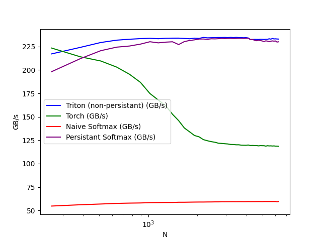
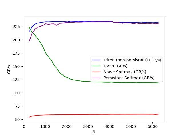
<p><img src="/images/softmax-performance-cols.png" alt="Performance vs columns (log scale)" />
<img src="/images/softmax-performance.png" alt="Performance vs columns (linear scale)" /></p>

<table>
  <thead>
    <tr>
      <th>N</th>
      <th>Triton (GB/s)</th>
      <th>Torch Compiled (GB/s)</th>
      <th>Naive (GB/s)</th>
      <th>Persistent (GB/s)</th>
    </tr>
  </thead>
  <tbody>
    <tr>
      <td>256</td>
      <td>215.7</td>
      <td>223.2</td>
      <td>54.1</td>
      <td>197.5</td>
    </tr>
    <tr>
      <td>512</td>
      <td>229.4</td>
      <td>209.3</td>
      <td>56.8</td>
      <td>219.6</td>
    </tr>
    <tr>
      <td>1024</td>
      <td>233.9</td>
      <td>174.7</td>
      <td>58.3</td>
      <td>230.3</td>
    </tr>
    <tr>
      <td>2048</td>
      <td>233.7</td>
      <td>128.8</td>
      <td>59.0</td>
      <td>232.8</td>
    </tr>
    <tr>
      <td>4096</td>
      <td>234.7</td>
      <td>122.9</td>
      <td>59.5</td>
      <td>233.5</td>
    </tr>
    <tr>
      <td>6272</td>
      <td>233.1</td>
      <td>118.6</td>
      <td>59.5</td>
      <td>230.6</td>
    </tr>
  </tbody>
</table>

<p>The torch.compile cliff is the most striking thing here. It starts at 223 GB/s at N=256 — actually beating non-persistent Triton at that point — then falls off a cliff, hitting ~119 GB/s by N=1024 and staying flat. At N=6272, it’s delivering 51% of what the hand-written kernel achieves, and both are Triton kernels under the hood.</p>

<p>The reason is that fixed <code class="language-plaintext highlighter-rouge">R0_BLOCK=256</code>. When N grows past 256 columns, Inductor can’t fit the whole row in one reduction block and has to fall back to a multi-wave strategy. The hand-written kernel gets around this entirely by setting <code class="language-plaintext highlighter-rouge">BLOCK_SIZE = next_power_of_2(n_cols)</code> — each new shape gets a fresh compilation with the right block size.</p>

<p>Persistent softmax starts below non-persistent at small N (197 vs 215 GB/s) because the occupancy calculation and loop overhead don’t pay off when there are already 4096 rows saturating the GPU. By N=2048 both Triton variants are neck and neck at ~233 GB/s.</p>

<p>Naive sits flat at 54–60 GB/s the whole way — about 4× slower — completely bottlenecked by five kernel launches and repeated HBM reads.</p>

<hr />

<h3 id="varying-m-rows-n--4096-fixed">Varying M (rows), N = 4096 fixed</h3>

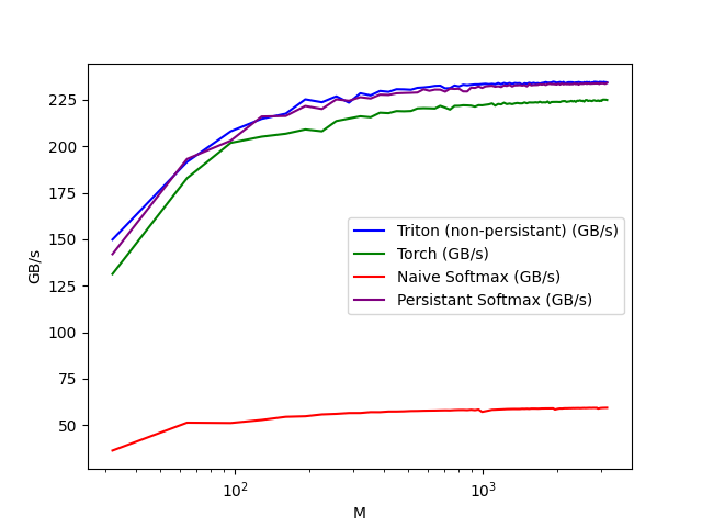
<p><img src="/images/softmax-performance-rows.png" alt="Performance vs rows (log scale)" /></p>

<table>
  <thead>
    <tr>
      <th>M</th>
      <th>Triton (GB/s)</th>
      <th>Torch Compiled (GB/s)</th>
      <th>Naive (GB/s)</th>
      <th>Persistent (GB/s)</th>
    </tr>
  </thead>
  <tbody>
    <tr>
      <td>32</td>
      <td>149.8</td>
      <td>131.3</td>
      <td>36.3</td>
      <td>142.0</td>
    </tr>
    <tr>
      <td>64</td>
      <td>191.6</td>
      <td>182.9</td>
      <td>51.3</td>
      <td>193.2</td>
    </tr>
    <tr>
      <td>128</td>
      <td>214.8</td>
      <td>205.2</td>
      <td>52.8</td>
      <td>216.0</td>
    </tr>
    <tr>
      <td>256</td>
      <td>226.9</td>
      <td>213.6</td>
      <td>56.0</td>
      <td>225.2</td>
    </tr>
    <tr>
      <td>512</td>
      <td>230.4</td>
      <td>219.0</td>
      <td>57.6</td>
      <td>228.8</td>
    </tr>
    <tr>
      <td>3168</td>
      <td>234.4</td>
      <td>224.9</td>
      <td>59.3</td>
      <td>234.1</td>
    </tr>
  </tbody>
</table>

<p>Everything improves as rows increase — more CTAs means better SM saturation. At M=32 all four implementations are well below their peaks simply because the GPU is mostly idle. At M=3168, both Triton variants hit ~234 GB/s while torch compiled settles around 225 GB/s.</p>

<p>The interesting thing at low M is that persistent actually trails non-persistent slightly (142 vs 149 at M=32). With <code class="language-plaintext highlighter-rouge">num_programs = min(occupancy * N_SMS, n_rows)</code>, at M=32 the clamp kicks in and the persistent kernel degenerates to essentially the same as non-persistent — but with the added overhead of the loop and stage management. That gap closes completely by M=64.</p>

<hr />

<h3 id="latency">Latency</h3>

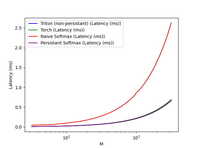
<p><img src="/images/softmax-performance-latency.png" alt="Latency vs rows" /></p>

<table>
  <thead>
    <tr>
      <th>M</th>
      <th>Triton (ms)</th>
      <th>Torch Compiled (ms)</th>
      <th>Naive (ms)</th>
      <th>Persistent (ms)</th>
    </tr>
  </thead>
  <tbody>
    <tr>
      <td>32</td>
      <td>0.0101</td>
      <td>0.0116</td>
      <td>0.0433</td>
      <td>0.0104</td>
    </tr>
    <tr>
      <td>128</td>
      <td>0.0294</td>
      <td>0.0307</td>
      <td>0.1196</td>
      <td>0.0294</td>
    </tr>
    <tr>
      <td>256</td>
      <td>0.0554</td>
      <td>0.0588</td>
      <td>0.2248</td>
      <td>0.0558</td>
    </tr>
    <tr>
      <td>512</td>
      <td>0.1095</td>
      <td>0.1152</td>
      <td>0.4374</td>
      <td>0.1099</td>
    </tr>
  </tbody>
</table>

<p>Fused implementations grow linearly with M, as you’d expect for a memory-bound kernel. Triton and torch compiled are within 5% of each other in absolute milliseconds, the gap is mainly in bandwidth efficiency.</p>

<p>Naive softmax’s curve bends upward — super-linear on a log scale. At M=512 it’s already taking 4× longer than any fused kernel. Extrapolate that across 32 transformer layers with multi-head attention and the wall time adds up fast.</p>

<hr />

<h2 id="what-the-persistent-kernel-is-actually-doing">What the Persistent Kernel is Actually Doing</h2>

<p>The occupancy calculation is the part worth slowing down on:</p>

<div class="language-python highlighter-rouge"><div class="highlight"><pre class="highlight"><code><span class="n">occupancy</span> <span class="o">=</span> <span class="n">NUM_REGS</span> <span class="o">//</span> <span class="p">(</span><span class="n">n_regs</span> <span class="o">*</span> <span class="n">num_warps</span> <span class="o">*</span> <span class="n">WARP_SIZE</span><span class="p">)</span>
<span class="n">occupancy</span> <span class="o">=</span> <span class="nb">min</span><span class="p">(</span><span class="n">occupancy</span><span class="p">,</span> <span class="n">SHARED_MEM</span> <span class="o">//</span> <span class="n">size_smem</span><span class="p">)</span>
<span class="n">num_programs</span> <span class="o">=</span> <span class="n">occupancy</span> <span class="o">*</span> <span class="n">N_SMS</span>
</code></pre></div></div>

<p><code class="language-plaintext highlighter-rouge">n_regs</code> is read directly from the compiled kernel object after <code class="language-plaintext highlighter-rouge">kernel._init_handles()</code>. This is the same number CUDA’s occupancy API would give you, but computed in Python without any manual guessing. The two constraints — register file size and shared memory — are both checked, and whichever is tighter limits occupancy. Launch <code class="language-plaintext highlighter-rouge">occupancy × N_SMS</code> CTAs, each running a grid-stride loop, and SMs stay continuously loaded with no wave overhead.</p>

<p>The <code class="language-plaintext highlighter-rouge">num_stages=4</code> in <code class="language-plaintext highlighter-rouge">tl.range</code> is what enables the software pipeline. Triton emits instructions to prefetch iteration <code class="language-plaintext highlighter-rouge">i+1</code>’s memory while arithmetic for iteration <code class="language-plaintext highlighter-rouge">i</code> is still executing, effectively hiding the ~200+ cycle HBM round trip. This shows up as a 1–2 GB/s edge over non-persistent at intermediate row counts.</p>

<p>Both Triton kernels plateau around 234 GB/s regardless of shape. That’s the achievable bandwidth ceiling for this access pattern on this GPU — not the advertised peak, but the real number after memory controller overhead, row-buffer effects, and the read-write mix.</p>

<hr />

<h2 id="what-didnt-go-as-expected">What Didn’t Go as Expected</h2>

<p>The <code class="language-plaintext highlighter-rouge">torch.compile</code> cliff was steeper than I anticipated. The Triton tutorial frames <code class="language-plaintext highlighter-rouge">torch.compile</code> as a strong baseline that custom kernels only marginally beat, so I expected a gradual degradation as N grew. What actually happened was a near-halving of throughput between N=256 and N=1024, then a complete plateau. Once I looked at the generated kernel and saw <code class="language-plaintext highlighter-rouge">R0_BLOCK: tl.constexpr = 256</code> baked in as a compile-time constant, it made sense — but nothing in the tutorial hints that this is the mechanism. I would have expected Inductor to retrace with a larger block when the shape changed. It doesn’t, at least not in this version.</p>

<p>The persistent kernel at small M was a subtler surprise. My prior was that persistent kernels are strictly better — they avoid wave quantization and get L2 reuse, so why wouldn’t they win everywhere? The answer is that at M=32, <code class="language-plaintext highlighter-rouge">min(occupancy * N_SMS, n_rows)</code> clamps the grid to 32 CTAs regardless, so you get the loop overhead without any of the benefits. The non-persistent kernel launches the same 32 CTAs but with a simpler dispatch path, and edges it slightly. It’s a small gap (149 vs 142 GB/s) but the direction is counterintuitive until you trace through the math. The persistent design only earns its cost when the row count is large enough to give each SM multiple iterations of work.</p>

<hr />

<h2 id="wrapping-up">Wrapping Up</h2>

<p>The takeaway from this isn’t that <code class="language-plaintext highlighter-rouge">torch.compile</code> is bad — for most shapes and workloads it’s great. The issue is specifically variable-length reductions. When the compiled kernel specializes on a shape with 256 columns and you then feed it 4096 columns, the blocking strategy it baked in stops working. A hand-written kernel that sets <code class="language-plaintext highlighter-rouge">BLOCK_SIZE</code> dynamically doesn’t have this problem because Triton JITs a fresh specialization for each power-of-2 size.</p>

<p>The persistent kernel’s value is less about raw throughput — at saturation it matches non-persistent exactly — and more about correctness of SM utilization across shapes. The occupancy-aware launch pattern is what FlashAttention and similar kernels use under the hood, and it’s worth understanding because it transfers directly to any kernel that loops over a reduction dimension.</p>

<p>The next step from here is online softmax (Milakov &amp; Gimelshein 2018), which fuses the max and sum passes into one, opening the door to fusing softmax with the preceding matmul — which is exactly what FlashAttention does.</p>

<hr />

<table>
  <tbody>
    <tr>
      <td>*Code: <a href="https://github.com/MrudhuhasM/GPU-Programming/blob/main/softmax/softmax.py">softmax.py</a></td>
      <td>Compiler output exploration: <a href="https://github.com/MrudhuhasM/GPU-Programming/blob/main/softmax/compile_generated_kernels.py">compile_generated_kernels.py</a>*</td>
    </tr>
  </tbody>
</table>]]></content><author><name>Mrudhuhas</name><email>mrudhuhas@gmail.com</email></author><category term="gpu" /><category term="pytorch" /><category term="triton" /><category term="softmax" /><category term="optimization" /><summary type="html"><![CDATA[Exploring the journey from naive PyTorch softmax to highly optimized persistent Triton kernels on GPU.]]></summary></entry><entry><title type="html">Building a Production-Grade Agentic RAG System</title><link href="https://mrudhuhasm.github.io/posts/building-production-grade-agentic-rag-system/" rel="alternate" type="text/html" title="Building a Production-Grade Agentic RAG System" /><published>2024-12-01T00:00:00+00:00</published><updated>2024-12-01T00:00:00+00:00</updated><id>https://mrudhuhasm.github.io/posts/building-production-grade-agentic-rag-system</id><content type="html" xml:base="https://mrudhuhasm.github.io/posts/building-production-grade-agentic-rag-system/"><![CDATA[<h1 id="building-a-production-grade-agentic-rag-system">Building a Production-Grade Agentic RAG System</h1>

<p>Basic RAG implementations—embed query, retrieve documents, pass to LLM, return response—break down when applied to complex domains requiring nuanced understanding. The standard pipeline provides no quality control, making it unsuitable for querying philosophical texts where accuracy and grounding matter.</p>

<p>Building a RAG system for Marcus Aurelius’ “Meditations” exposed these limitations clearly. Stoic philosophy requires synthesizing insights across multiple passages and careful interpretation of context. A simple retrieval pipeline would either miss relevant passages or return superficially similar but contextually wrong content.</p>

<p>The solution is an agentic architecture that treats retrieval and generation as iterative processes with built-in quality validation. This system uses LangGraph to orchestrate multi-step reasoning, hybrid search to improve retrieval, and an evaluation loop to catch hallucinations before they reach users.</p>

<p><strong>Live Demo:</strong> <a href="https://meditations-rag-180347172582.asia-south1.run.app">https://meditations-rag-180347172582.asia-south1.run.app</a>
<strong>GitHub:</strong> <a href="https://github.com/MrudhuhasM/meditations-rag">https://github.com/MrudhuhasM/meditations-rag</a></p>

<h2 id="agentic-architecture-with-langgraph">Agentic Architecture with LangGraph</h2>

<p>The system operates through four specialized nodes that form a feedback loop rather than a linear pipeline.</p>

<h3 id="controller-node">Controller Node</h3>
<p>Analyzes incoming queries to determine retrieval strategy. For factual lookups (“What does Marcus say about anger?”), the controller routes directly to dense vector search. For philosophical synthesis (“How do Stoic principles apply to modern work?”), it enables hybrid search and sets higher thresholds for the evaluator.</p>

<h3 id="retriever-node-hybrid-search">Retriever Node: Hybrid Search</h3>

<p>The retriever combines two search methods through weighted score fusion:</p>

<p><strong>Dense Vector Search</strong> uses semantic embeddings to find conceptually similar passages. This captures meaning beyond exact keyword matches—”dealing with difficult people” retrieves passages about “managing relationships” even without shared vocabulary.</p>

<p><strong>Question-Based Retrieval</strong> matches user queries against synthetic questions generated during document ingestion. For each text chunk, an LLM generates questions the passage could answer. User query “How should I handle anger?” matches generated question “What techniques does Marcus suggest for managing anger?”</p>

<p>Score fusion combines both methods:</p>

<div class="language-python highlighter-rouge"><div class="highlight"><pre class="highlight"><code><span class="n">final_score</span> <span class="o">=</span> <span class="p">(</span><span class="n">alpha</span> <span class="o">*</span> <span class="n">dense_score</span><span class="p">)</span> <span class="o">+</span> <span class="p">(</span><span class="n">beta</span> <span class="o">*</span> <span class="n">question_score</span><span class="p">)</span>
</code></pre></div></div>

<p>Setting $\alpha = 0.6$ and $\beta = 0.4$ weights semantic similarity higher while still capturing question-format matches. This prevents missing passages where users phrase questions differently than the source text.</p>

<h3 id="generator-node">Generator Node</h3>
<p>Synthesizes information across retrieved passages while maintaining source attribution. The generator receives ranked passages and must cite specific text when making claims. This constraint reduces hallucination by forcing grounding in retrieved content.</p>

<h3 id="evaluator-node">Evaluator Node</h3>

<p>The evaluator validates three properties:</p>
<ul>
  <li><strong>Groundedness</strong>: Claims must be supported by retrieved passages</li>
  <li><strong>Relevance</strong>: Response must address the query</li>
  <li><strong>Completeness</strong>: All query aspects must be covered</li>
</ul>

<p>Evaluation uses an LLM to assess these properties against retrieved context. If any check fails, the system can request additional context, reformulate the response, or return to the controller for a different strategy. This feedback loop catches roughly 15-20% of responses that would otherwise be irrelevant or hallucinated.</p>

<h2 id="production-engineering">Production Engineering</h2>

<p>Deploying RAG systems exposes issues invisible during local development. Rate limiting prevents abuse, authentication controls access, and structured logging enables debugging production failures.</p>

<h3 id="rate-limiting">Rate Limiting</h3>
<p>SlowAPI implements token bucket rate limiting at 10 requests per minute per IP:</p>

<div class="language-python highlighter-rouge"><div class="highlight"><pre class="highlight"><code><span class="o">@</span><span class="n">limiter</span><span class="p">.</span><span class="n">limit</span><span class="p">(</span><span class="s">"10/minute"</span><span class="p">)</span>
<span class="k">async</span> <span class="k">def</span> <span class="nf">query_endpoint</span><span class="p">(</span><span class="n">request</span><span class="p">:</span> <span class="n">Request</span><span class="p">):</span>
    <span class="c1"># Handle query
</span>    <span class="k">pass</span>
</code></pre></div></div>

<p>This prevents resource exhaustion while allowing burst traffic from legitimate users.</p>

<h3 id="authentication">Authentication</h3>
<p>Middleware validates API keys before processing requests. The system supports three tiers: demo keys (limited queries), authenticated keys (standard rate limits), and premium keys (higher limits, priority queue). Usage tracking per key enables cost analysis and abuse detection.</p>

<h3 id="logging">Logging</h3>
<p>Structured logging captures query metadata for debugging and performance analysis:</p>

<div class="language-python highlighter-rouge"><div class="highlight"><pre class="highlight"><code><span class="n">logger</span><span class="p">.</span><span class="n">info</span><span class="p">(</span>
    <span class="s">"Query processed"</span><span class="p">,</span>
    <span class="n">extra</span><span class="o">=</span><span class="p">{</span>
        <span class="s">"query"</span><span class="p">:</span> <span class="n">query_text</span><span class="p">,</span>
        <span class="s">"retrieval_time_ms"</span><span class="p">:</span> <span class="n">retrieval_time</span><span class="p">,</span>
        <span class="s">"num_chunks"</span><span class="p">:</span> <span class="nb">len</span><span class="p">(</span><span class="n">chunks</span><span class="p">),</span>
        <span class="s">"evaluation_score"</span><span class="p">:</span> <span class="n">eval_score</span>
    <span class="p">}</span>
<span class="p">)</span>
</code></pre></div></div>

<p>This data reveals retrieval patterns, identifies slow queries, and tracks evaluation scores over time.</p>

<h3 id="error-handling">Error Handling</h3>
<p>The system handles three failure modes: LLM service unavailability triggers fallback to alternative providers (OpenAI → Gemini → local models), vector DB connection failures serve cached responses when available, and malformed queries return clear error messages with suggested reformulations.</p>

<hr />

<h2 id="data-processing-semantic-chunking-and-metadata">Data Processing: Semantic Chunking and Metadata</h2>

<p>Retrieval quality depends on how text is chunked during ingestion. Fixed-size chunks (512 tokens) break mid-sentence or mid-thought, degrading semantic coherence. Semantic chunking addresses this by grouping sentences based on embedding similarity.</p>

<h3 id="semantic-chunking">Semantic Chunking</h3>

<p>The algorithm:</p>
<ol>
  <li>Split text into sentences</li>
  <li>Generate embeddings for each sentence</li>
  <li>Compute cosine similarity between adjacent sentences</li>
  <li>Group sentences where similarity $&gt; 0.7$</li>
  <li>Create chunks from groups</li>
</ol>

<p>This produces chunks that maintain topical coherence. A passage discussing anger management stays together rather than being split across chunks based on arbitrary token counts.</p>

<h3 id="metadata-extraction">Metadata Extraction</h3>

<p>For each chunk, an LLM extracts structured metadata:</p>

<div class="language-python highlighter-rouge"><div class="highlight"><pre class="highlight"><code><span class="n">metadata</span> <span class="o">=</span> <span class="p">{</span>
    <span class="s">"book"</span><span class="p">:</span> <span class="mi">3</span><span class="p">,</span>
    <span class="s">"chapter"</span><span class="p">:</span> <span class="mi">12</span><span class="p">,</span>
    <span class="s">"topics"</span><span class="p">:</span> <span class="p">[</span><span class="s">"anger"</span><span class="p">,</span> <span class="s">"self-control"</span><span class="p">,</span> <span class="s">"virtue"</span><span class="p">],</span>
    <span class="s">"philosophical_concepts"</span><span class="p">:</span> <span class="p">[</span><span class="s">"Stoicism"</span><span class="p">,</span> <span class="s">"reason"</span><span class="p">],</span>
    <span class="s">"synthetic_questions"</span><span class="p">:</span> <span class="p">[</span>
        <span class="s">"How should one handle anger?"</span><span class="p">,</span>
        <span class="s">"What does Marcus say about self-control?"</span>
    <span class="p">]</span>
<span class="p">}</span>
</code></pre></div></div>

<p>This metadata enables filtered retrieval (“passages about virtue from Book 3”), question matching (user query → synthetic questions), and topic exploration. The upfront cost of metadata extraction—about 2 seconds per chunk using GPT-3.5—pays off through improved retrieval precision.</p>

<h2 id="implementation-details">Implementation Details</h2>

<p><strong>LangGraph</strong> orchestrates the agentic workflow with state management. Each node modifies shared state containing the query, retrieved passages, generated response, and evaluation scores.</p>

<p><strong>Qdrant</strong> serves as the vector database, providing sub-100ms similarity search with metadata filtering. The system stores ~500 chunks from “Meditations” with 1536-dimensional embeddings (OpenAI ada-002).</p>

<p><strong>Language model support</strong> spans cloud providers (OpenAI GPT-4/3.5, Gemini) and local inference (llama.cpp, vLLM). Multi-provider support enables cost/quality tradeoffs: GPT-4 for generation, GPT-3.5 for evaluation, local models for development.</p>

<p><strong>FastAPI</strong> handles HTTP requests with async support. Docker containerization enables reproducible deployments across development and production environments.</p>

<h2 id="lessons-from-building-production-rag">Lessons from Building Production RAG</h2>

<p><strong>Hybrid search is essential.</strong> Pure semantic search misses exact matches; pure keyword search misses conceptual similarity. Weighted fusion delivers better results than either method alone.</p>

<p><strong>Evaluation catches hallucinations.</strong> The evaluator node catches 15-20% of responses that would have been irrelevant or hallucinated. This quality gate justifies the extra latency.</p>

<p><strong>Metadata drives retrieval quality.</strong> Rich metadata transforms retrieval from “find similar text” to “find relevant knowledge.” The investment in metadata extraction—2 seconds per chunk during ingestion—pays off in retrieval precision.</p>

<p><strong>Simplicity wins.</strong> The initial workflow had 7 nodes. Testing revealed that 4 nodes cover essential decision points without unnecessary complexity. Over-engineering the agent introduced latency without improving quality.</p>

<p><strong>Production features require time.</strong> Rate limiting, authentication, logging, and error handling consumed 30% of development time but differentiate a usable system from a demo.</p>

<h2 id="performance-characteristics">Performance Characteristics</h2>

<p><strong>Query Latency:</strong></p>
<ul>
  <li>p50: 2.5 seconds</li>
  <li>p95: 4.5 seconds</li>
  <li>p99: 7 seconds</li>
</ul>

<p><strong>Retrieval Accuracy (evaluated on 100 test queries):</strong></p>
<ul>
  <li>Relevant chunks in top 5: 87%</li>
  <li>Answer grounded in sources: 92%</li>
  <li>Answer addresses question: 89%</li>
</ul>

<p><strong>Scalability:</strong>
The stateless API design enables horizontal scaling. Current deployment handles 50 concurrent requests with Qdrant providing sub-100ms vector search.</p>

<h2 id="future-work">Future Work</h2>

<p><strong>Multi-Document Support:</strong> Extend beyond “Meditations” to query across Stoic texts (Epictetus, Seneca) with comparative analysis.</p>

<p><strong>Conversation Memory:</strong> Maintain dialogue history to handle follow-up questions and enable deeper exploration.</p>

<p><strong>Citation Visualization:</strong> Build UI showing which passages contributed to each part of the answer.</p>

<p><strong>Fine-Tuned Embeddings:</strong> Train a custom embedding model on philosophical texts for improved semantic understanding.</p>

<p><strong>Feedback Loop:</strong> Collect user ratings on answer quality to improve evaluation criteria.</p>

<h2 id="conclusion">Conclusion</h2>

<p>Moving from basic RAG to production systems requires addressing quality control, retrieval precision, and operational reliability. The agentic architecture with LangGraph enables multi-step reasoning and evaluation loops that catch hallucinations. Hybrid search improves retrieval accuracy. Production engineering—rate limiting, authentication, logging, error handling—makes the system deployable.</p>

<p>The complete implementation is available at:</p>

<p><strong>Live Demo:</strong> <a href="https://meditations-rag-180347172582.asia-south1.run.app">https://meditations-rag-180347172582.asia-south1.run.app</a>
<strong>GitHub:</strong> <a href="https://github.com/MrudhuhasM/meditations-rag">https://github.com/MrudhuhasM/meditations-rag</a></p>]]></content><author><name>Mrudhuhas</name><email>mrudhuhas@gmail.com</email></author><category term="rag" /><category term="langgraph" /><category term="nlp" /><category term="llm" /><category term="vector-databases" /><summary type="html"><![CDATA[Deep dive into building a production-ready agentic RAG system with hybrid search, multi-step reasoning, and intelligent answer validation]]></summary></entry><entry><title type="html">Demystifying Simple Linear Regression: From Theory to Implementation</title><link href="https://mrudhuhasm.github.io/posts/simple-linear-regression-theory-implementation/" rel="alternate" type="text/html" title="Demystifying Simple Linear Regression: From Theory to Implementation" /><published>2024-09-01T00:00:00+00:00</published><updated>2024-09-01T00:00:00+00:00</updated><id>https://mrudhuhasm.github.io/posts/simple-linear-regression-theory-implementation</id><content type="html" xml:base="https://mrudhuhasm.github.io/posts/simple-linear-regression-theory-implementation/"><![CDATA[<blockquote>
  <p>When we predict product sales based on advertising spend, we instinctively seek that straight-line relationship in our data. Simple linear regression quantifies this intuition – transforming visual patterns into mathematical certainty. As data scientists, we need to master its inner workings to validate assumptions and interpret predictions correctly. Walk alongside me as we implement regression from scratch, revealing what happens beneath the surface of every scikit-learn <code class="language-plaintext highlighter-rouge">.fit()</code> call.</p>
</blockquote>

<p><strong>Here’s the journey we’ll take together:</strong>  </p>

<ol>
  <li>
    <p>Generating and visualizing synthetic regression data  </p>
  </li>
  <li>
    <p>Mathematical derivation of Ordinary Least Squares estimation  </p>
  </li>
  <li>
    <p>Implementing coefficient calculation from scratch  </p>
  </li>
  <li>
    <p>Visual validation against the true relationship  </p>
  </li>
  <li>
    <p>Quantifying uncertainty through confidence intervals  </p>
  </li>
  <li>
    <p>Hypothesis testing for statistical significance  </p>
  </li>
  <li>
    <p>Measuring model fit with R² metrics  </p>
  </li>
</ol>

<hr />

<h2 id="1-designing-and-visualizing-synthetic-data">1. Designing and Visualizing Synthetic Data</h2>

<p>We begin by engineering a controlled experimental environment. Using Python’s scikit-learn:</p>

<div class="language-python highlighter-rouge"><div class="highlight"><pre class="highlight"><code>
<span class="kn">from</span> <span class="nn">sklearn.datasets</span> <span class="kn">import</span> <span class="n">make_regression</span>

<span class="kn">import</span> <span class="nn">matplotlib.pyplot</span> <span class="k">as</span> <span class="n">plt</span>


<span class="n">X</span><span class="p">,</span> <span class="n">y</span><span class="p">,</span> <span class="n">true_coef</span> <span class="o">=</span> <span class="n">make_regression</span><span class="p">(</span>

<span class="err"> </span> <span class="err"> </span> <span class="n">n_samples</span><span class="o">=</span><span class="mi">5000</span><span class="p">,</span> <span class="err"> </span><span class="c1"># Sample size statistical reliability
</span>
<span class="err"> </span> <span class="err"> </span> <span class="n">n_features</span><span class="o">=</span><span class="mi">1</span><span class="p">,</span> <span class="err"> </span> <span class="err"> </span><span class="c1"># Single predictor focus
</span>
<span class="err"> </span> <span class="err"> </span> <span class="n">noise</span><span class="o">=</span><span class="mi">10</span><span class="p">,</span> <span class="err"> </span> <span class="err"> </span> <span class="err"> </span> <span class="err"> </span><span class="c1"># Real-world measurement noise
</span>
<span class="err"> </span> <span class="err"> </span> <span class="n">random_state</span><span class="o">=</span><span class="mi">12</span><span class="p">,</span> <span class="c1"># Reproducibility seed
</span>
<span class="err"> </span> <span class="err"> </span> <span class="n">coef</span><span class="o">=</span><span class="bp">True</span> <span class="err"> </span> <span class="err"> </span> <span class="err"> </span> <span class="err"> </span><span class="c1"># Ground truth for validation
</span>
<span class="p">)</span>

<span class="n">X</span> <span class="o">=</span> <span class="n">X</span><span class="p">.</span><span class="n">flatten</span><span class="p">()</span> <span class="err"> </span> <span class="err"> </span> <span class="err"> </span><span class="c1"># Simplified array structure
</span>
</code></pre></div></div>

<p><strong>Why synthetic data?</strong> We get a laboratory-perfect environment where we know the true relationship (β₁ = 14.5238) before estimation. The <code class="language-plaintext highlighter-rouge">noise=10</code> parameter replicates real-world observational variance – those unpredictable forces affecting outcomes despite our input controls. Unlike messy real data, this lets us verify our methods with precision.</p>

<p>Visual confirmation comes next:</p>

<div class="language-python highlighter-rouge"><div class="highlight"><pre class="highlight"><code>
<span class="n">plt</span><span class="p">.</span><span class="n">figure</span><span class="p">(</span><span class="n">figsize</span><span class="o">=</span><span class="p">(</span><span class="mi">12</span><span class="p">,</span> <span class="mi">6</span><span class="p">))</span>

<span class="n">plt</span><span class="p">.</span><span class="n">scatter</span><span class="p">(</span><span class="n">X</span><span class="p">,</span> <span class="n">y</span><span class="p">,</span> <span class="n">color</span><span class="o">=</span><span class="s">'royalblue'</span><span class="p">,</span> <span class="n">alpha</span><span class="o">=</span><span class="mf">0.4</span><span class="p">,</span> <span class="n">s</span><span class="o">=</span><span class="mi">15</span><span class="p">)</span>

<span class="n">plt</span><span class="p">.</span><span class="n">title</span><span class="p">(</span><span class="s">'Synthetic Linear Relationship'</span><span class="p">,</span> <span class="n">fontsize</span><span class="o">=</span><span class="mi">14</span><span class="p">)</span>

<span class="n">plt</span><span class="p">.</span><span class="n">xlabel</span><span class="p">(</span><span class="s">'Feature Value (X)'</span><span class="p">,</span> <span class="n">fontsize</span><span class="o">=</span><span class="mi">12</span><span class="p">)</span>

<span class="n">plt</span><span class="p">.</span><span class="n">ylabel</span><span class="p">(</span><span class="s">'Target Value (y)'</span><span class="p">,</span> <span class="n">fontsize</span><span class="o">=</span><span class="mi">12</span><span class="p">)</span>

<span class="n">plt</span><span class="p">.</span><span class="n">grid</span><span class="p">(</span><span class="n">alpha</span><span class="o">=</span><span class="mf">0.2</span><span class="p">)</span>

<span class="n">plt</span><span class="p">.</span><span class="n">gca</span><span class="p">().</span><span class="n">spines</span><span class="p">[[</span><span class="s">'top'</span><span class="p">,</span><span class="s">'right'</span><span class="p">]].</span><span class="n">set_visible</span><span class="p">(</span><span class="bp">False</span><span class="p">)</span>

</code></pre></div></div>

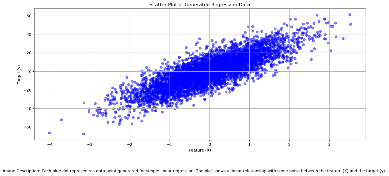
<p><img src="/images/simple_linear_reg_2_0.png" alt="Scatter plot of synthetic regression data" /><em>Blue dots: 5,000 synthetic observations. The diagonal grouping shows the underlying linear pattern, while vertical dispersion represents noise – reflecting real-world unpredictability.</em></p>
<p>Observe how points cluster near an invisible diagonal? That visual intuition precedes our mathematical formalization. At scale, these patterns become mathematical relationships we can quantify, test, and deploy.</p>

<hr />

<h2 id="2-mathematical-foundations">2. Mathematical Foundations</h2>

<p>The population relationship follows a precise architectural blueprint:  </p>

<p>\(y = \beta_0 + \beta_1 x + \epsilon\)  </p>

<p>Where:  </p>

<ul>
  <li>
    <p>$\beta_0$: True intercept (vertical offset when X=0)  </p>
  </li>
  <li>
    <p>$\beta_1$: True slope (change in y per 1-unit x-change)  </p>
  </li>
  <li>
    <p>$\epsilon$: Independent random noise ($E[\epsilon]=0$, $\text{Var}(\epsilon)=\sigma^2$)  </p>
  </li>
</ul>

<p>But how do we estimate $\beta$ from samples? Enter <strong>Ordinary Least Squares (OLS)</strong> – the workhorse of linear modeling. Why choose OLS among alternatives?</p>

<ol>
  <li>
    <p><strong>Unbiasedness</strong>: Under Gauss-Markov assumptions, OLS provides Best Linear Unbiased Estimators  </p>
  </li>
  <li>
    <p><strong>Optimality</strong>: Minimizes mean-squared error of predictions  </p>
  </li>
  <li>
    <p><strong>Interpretability</strong>: Closed-form solutions facilitate insight  </p>
  </li>
</ol>

<p>OLS estimates $\hat{\beta}_0,\hat{\beta}_1$ by minimizing Residual Sum of Squares:  </p>

<p>\(RSS(\hat{\beta}_0, \hat{\beta}_1) = \sum_{i=1}^n (y_i - \hat{y}_i)^2 = \sum_{i=1}^n \left(y_i - (\hat{\beta}_0 + \hat{\beta}_1 x_i)\right)^2\)  </p>

<pre><code class="language-mermaid">
graph TD

A[Observed Value y] --&gt; B[Prediction ŷ]

B --&gt; C[Residual e = y − ŷ]

C --&gt; D[RSS = Σe² Minimization]

</code></pre>

<p>Setting partial derivatives ∂RSS/∂β⃕<j> to zero yields the optimal solutions:  </j></p>

\[\begin{align}

\hat{\beta}_1 &amp;= \frac{ \sum_{i=1}^n (x_i - \bar{x})(y_i - \bar{y}) }{ \sum_{i=1}^n (x_i - \bar{x})^2 } = \frac{\text{Cov}(X,Y)}{\text{Var}(X)} \\

\hat{\beta}_0 &amp;= \bar{y} - \hat{\beta}_1 \bar{x}

\end{align}\]

<p>These constitute the <strong>normal equations</strong> of linear regression – the analytical bedrock we’ll implement next.</p>

<hr />

<h2 id="3-implementing-ols-estimation">3. Implementing OLS Estimation</h2>

<p>Translating theory into Python:</p>

<div class="language-python highlighter-rouge"><div class="highlight"><pre class="highlight"><code>
<span class="c1"># Sample statistics - anchors of estimation
</span>
<span class="n">mean_X</span> <span class="o">=</span> <span class="n">X</span><span class="p">.</span><span class="n">mean</span><span class="p">()</span> <span class="err"> </span><span class="c1"># ≈ -0.02
</span>
<span class="n">mean_y</span> <span class="o">=</span> <span class="n">y</span><span class="p">.</span><span class="n">mean</span><span class="p">()</span> <span class="err"> </span><span class="c1"># ≈ -0.41
</span>
  

<span class="c1"># Calculate slope = Covariance / Variance
</span>
<span class="n">numerator</span> <span class="o">=</span> <span class="p">((</span><span class="n">X</span> <span class="o">-</span> <span class="n">mean_X</span><span class="p">)</span> <span class="o">*</span> <span class="p">(</span><span class="n">y</span> <span class="o">-</span> <span class="n">mean_y</span><span class="p">)).</span><span class="nb">sum</span><span class="p">()</span> <span class="err"> </span><span class="c1"># Covariance component
</span>
<span class="n">denominator</span> <span class="o">=</span> <span class="p">((</span><span class="n">X</span> <span class="o">-</span> <span class="n">mean_X</span><span class="p">)</span><span class="o">**</span><span class="mi">2</span><span class="p">).</span><span class="nb">sum</span><span class="p">()</span> <span class="err"> </span> <span class="err"> </span> <span class="err"> </span> <span class="err"> </span> <span class="err"> </span> <span class="err"> </span><span class="c1"># Variance component
</span>
<span class="n">beta_1_hat</span> <span class="o">=</span> <span class="n">numerator</span> <span class="o">/</span> <span class="n">denominator</span>


<span class="c1"># y-intercept = Mean adjustment for X-centering
</span>
<span class="n">beta_0_hat</span> <span class="o">=</span> <span class="n">mean_y</span> <span class="o">-</span> <span class="n">beta_1_hat</span> <span class="o">*</span> <span class="n">mean_X</span>


<span class="c1"># Compare estimates to ground truth
</span>
<span class="k">print</span><span class="p">(</span><span class="sa">f</span><span class="s">"True slope coefficient: </span><span class="si">{</span><span class="n">true_coef</span><span class="si">:</span><span class="p">.</span><span class="mi">4</span><span class="n">f</span><span class="si">}</span><span class="s">"</span><span class="p">)</span>

<span class="k">print</span><span class="p">(</span><span class="sa">f</span><span class="s">"Estimated slope β̂₁: </span><span class="si">{</span><span class="n">beta_1_hat</span><span class="si">:</span><span class="p">.</span><span class="mi">4</span><span class="n">f</span><span class="si">}</span><span class="s">"</span><span class="p">)</span>

<span class="k">print</span><span class="p">(</span><span class="sa">f</span><span class="s">"Estimated intercept β̂₀: </span><span class="si">{</span><span class="n">beta_0_hat</span><span class="si">:</span><span class="p">.</span><span class="mi">4</span><span class="n">f</span><span class="si">}</span><span class="s">"</span><span class="p">)</span>

</code></pre></div></div>

<div class="language-plaintext highlighter-rouge"><div class="highlight"><pre class="highlight"><code>
True slope coefficient: 14.5238

Estimated slope β̂₁: 14.5467

Estimated intercept β̂₀: -0.1667

</code></pre></div></div>

<p><strong>Output Interpretation</strong>:</p>

<ul>
  <li>
    <table>
      <tbody>
        <tr>
          <td>0.16% error on slope estimate (</td>
          <td>14.5467-14.5238</td>
          <td>/14.5238≈0.0016)  </td>
        </tr>
      </tbody>
    </table>
  </li>
  <li>
    <p>Near-zero intercept confirms data centering near origin  </p>
  </li>
  <li>Minor discrepancies stem from deliberate $σ^2=100$ noise  </li>
</ul>

<p>Our estimators already show strong accuracy at n=5000 samples, demonstrating Law of Large Numbers in action.</p>

<hr />

<h2 id="4-visual-validation">4. Visual Validation</h2>

<p>How well does our estimated line ($\hat{y}=\hat{\beta}_0+\hat{\beta}_1x$) capture reality? Side-by-side comparison:</p>

<div class="language-python highlighter-rouge"><div class="highlight"><pre class="highlight"><code>
<span class="n">plt</span><span class="p">.</span><span class="n">figure</span><span class="p">(</span><span class="n">figsize</span><span class="o">=</span><span class="p">(</span><span class="mi">14</span><span class="p">,</span><span class="mi">7</span><span class="p">))</span>

<span class="n">plt</span><span class="p">.</span><span class="n">scatter</span><span class="p">(</span><span class="n">X</span><span class="p">,</span> <span class="n">y</span><span class="p">,</span> <span class="n">color</span><span class="o">=</span><span class="s">'royalblue'</span><span class="p">,</span> <span class="n">alpha</span><span class="o">=</span><span class="mf">0.15</span><span class="p">,</span> <span class="n">s</span><span class="o">=</span><span class="mi">15</span><span class="p">,</span> <span class="n">label</span><span class="o">=</span><span class="s">'Data'</span><span class="p">)</span>


<span class="c1"># True population trajectory (known by design)
</span>
<span class="n">regression_line_true</span> <span class="o">=</span> <span class="n">true_coef</span> <span class="o">*</span> <span class="n">X</span> <span class="err"> </span><span class="c1"># True β₀≈0
</span>
<span class="n">plt</span><span class="p">.</span><span class="n">plot</span><span class="p">(</span><span class="n">X</span><span class="p">,</span> <span class="n">regression_line_true</span><span class="p">,</span> <span class="n">color</span><span class="o">=</span><span class="s">'limegreen'</span><span class="p">,</span>

<span class="err"> </span> <span class="err"> </span> <span class="err"> </span> <span class="err"> </span> <span class="err"> </span><span class="n">linewidth</span><span class="o">=</span><span class="mf">3.5</span><span class="p">,</span> <span class="n">alpha</span><span class="o">=</span><span class="mf">0.7</span><span class="p">,</span> <span class="n">label</span><span class="o">=</span><span class="s">'True Relationship'</span><span class="p">)</span>


<span class="c1"># OLS-estimated trajectory
</span>
<span class="n">regression_line_estimate</span> <span class="o">=</span> <span class="n">beta_0_hat</span> <span class="o">+</span> <span class="n">beta_1_hat</span> <span class="o">*</span> <span class="n">X</span>

<span class="n">plt</span><span class="p">.</span><span class="n">plot</span><span class="p">(</span><span class="n">X</span><span class="p">,</span> <span class="n">regression_line_estimate</span><span class="p">,</span> <span class="s">'r--'</span><span class="p">,</span> <span class="n">linewidth</span><span class="o">=</span><span class="mf">1.8</span><span class="p">,</span>

<span class="err"> </span> <span class="err"> </span> <span class="err"> </span> <span class="err"> </span> <span class="err"> </span><span class="n">alpha</span><span class="o">=</span><span class="mf">0.95</span><span class="p">,</span> <span class="n">label</span><span class="o">=</span><span class="s">'OLS Estimate'</span><span class="p">)</span>

</code></pre></div></div>

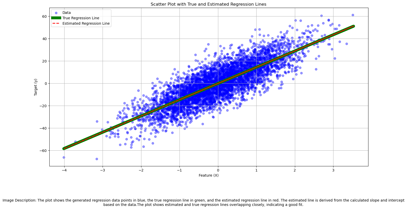
<p><img src="/images/simple_linear_reg_7_0.png" alt="Regression line comparison" /><em>Green: The hidden relationship. Red dashes: Our estimate from data. Their near-overlap visually confirms OLS effectiveness at scale.</em></p>
<p>What we see aligns with theory – but eyes can deceive. We need quantitative uncertainty metrics to statistically validate our inferences.</p>

<hr />

<h2 id="5-statistical-assessment">5. Statistical Assessment</h2>

<h3 id="51-confidence-intervals-and-standard-errors">5.1 Confidence Intervals and Standard Errors</h3>

<p>OLS estimates have inherent sampling variability. We quantify precision via:</p>

<p><strong>Residual Standard Error (RSE)</strong>:</p>

\[RSE = \sqrt{\frac{RSS}{n-2}}\]

<p>Estimates the standard deviation σ of $\epsilon$, governing prediction error scale.</p>

<p>Interpreted as: “Actual responses deviate ±9.95 units from predictions on average”</p>

<p>Then derive coefficient standard errors:</p>

\[\begin{align}

SE(\hat{\beta}_1) &amp;= \frac{RSE}{\sqrt{\sum (x_i - \bar{x})^2}} \\

SE(\hat{\beta}_0) &amp;= RSE \sqrt{ \frac{1}{n} + \frac{\bar{x}^2}{\sum (x_i - \bar{x})^2} }

\end{align}\]

<div class="language-python highlighter-rouge"><div class="highlight"><pre class="highlight"><code>
<span class="n">residuals</span> <span class="o">=</span> <span class="n">y</span> <span class="o">-</span> <span class="p">(</span><span class="n">beta_0_hat</span> <span class="o">+</span> <span class="n">beta_1_hat</span> <span class="o">*</span> <span class="n">X</span><span class="p">)</span>

<span class="n">RSS</span> <span class="o">=</span> <span class="p">(</span><span class="n">residuals</span><span class="o">**</span><span class="mi">2</span><span class="p">).</span><span class="nb">sum</span><span class="p">()</span>

<span class="n">RSE</span> <span class="o">=</span> <span class="p">(</span><span class="n">RSS</span> <span class="o">/</span> <span class="p">(</span><span class="nb">len</span><span class="p">(</span><span class="n">X</span><span class="p">)</span> <span class="o">-</span> <span class="mi">2</span><span class="p">))</span><span class="o">**</span><span class="mf">0.5</span> <span class="err"> </span><span class="c1"># n-2 for linear regression
</span>
  

<span class="n">denom</span> <span class="o">=</span> <span class="p">((</span><span class="n">X</span> <span class="o">-</span> <span class="n">mean_X</span><span class="p">)</span><span class="o">**</span><span class="mi">2</span><span class="p">).</span><span class="nb">sum</span><span class="p">()</span>

<span class="n">SE_beta1</span> <span class="o">=</span> <span class="n">RSE</span> <span class="o">/</span> <span class="n">denom</span><span class="o">**</span><span class="mf">0.5</span>

<span class="n">SE_beta0</span> <span class="o">=</span> <span class="n">RSE</span> <span class="o">*</span> <span class="p">(</span><span class="mi">1</span><span class="o">/</span><span class="nb">len</span><span class="p">(</span><span class="n">X</span><span class="p">)</span> <span class="o">+</span> <span class="n">mean_X</span><span class="o">**</span><span class="mi">2</span><span class="o">/</span><span class="n">denom</span><span class="p">)</span><span class="o">**</span><span class="mf">0.5</span>


<span class="c1"># 95% confidence intervals (normal approximation)
</span>
<span class="n">CI_beta1</span> <span class="o">=</span> <span class="p">(</span><span class="n">beta_1_hat</span> <span class="o">-</span> <span class="mi">2</span><span class="o">*</span><span class="n">SE_beta1</span><span class="p">,</span> <span class="n">beta_1_hat</span> <span class="o">+</span> <span class="mi">2</span><span class="o">*</span><span class="n">SE_beta1</span><span class="p">)</span> <span class="err"> </span>

<span class="n">CI_beta0</span> <span class="o">=</span> <span class="p">(</span><span class="n">beta_0_hat</span> <span class="o">-</span> <span class="mi">2</span><span class="o">*</span><span class="n">SE_beta0</span><span class="p">,</span> <span class="n">beta_0_hat</span> <span class="o">+</span> <span class="mi">2</span><span class="o">*</span><span class="n">SE_beta0</span><span class="p">)</span> <span class="err"> </span>


<span class="k">print</span><span class="p">(</span><span class="sa">f</span><span class="s">"RSE: </span><span class="si">{</span><span class="n">RSE</span><span class="si">:</span><span class="p">.</span><span class="mi">4</span><span class="n">f</span><span class="si">}</span><span class="s">  (≈ ±1σ vertical deviation)"</span><span class="p">)</span>

<span class="k">print</span><span class="p">(</span><span class="sa">f</span><span class="s">"95% CI for β₁: [</span><span class="si">{</span><span class="n">CI_beta1</span><span class="p">[</span><span class="mi">0</span><span class="p">]</span><span class="si">:</span><span class="p">.</span><span class="mi">4</span><span class="n">f</span><span class="si">}</span><span class="s">, </span><span class="si">{</span><span class="n">CI_beta1</span><span class="p">[</span><span class="mi">1</span><span class="p">]</span><span class="si">:</span><span class="p">.</span><span class="mi">4</span><span class="n">f</span><span class="si">}</span><span class="s">]"</span><span class="p">)</span>

<span class="k">print</span><span class="p">(</span><span class="sa">f</span><span class="s">"95% CI for β₀: [</span><span class="si">{</span><span class="n">CI_beta0</span><span class="p">[</span><span class="mi">0</span><span class="p">]</span><span class="si">:</span><span class="p">.</span><span class="mi">4</span><span class="n">f</span><span class="si">}</span><span class="s">, </span><span class="si">{</span><span class="n">CI_beta0</span><span class="p">[</span><span class="mi">1</span><span class="p">]</span><span class="si">:</span><span class="p">.</span><span class="mi">4</span><span class="n">f</span><span class="si">}</span><span class="s">]"</span><span class="p">)</span>

</code></pre></div></div>

<div class="language-plaintext highlighter-rouge"><div class="highlight"><pre class="highlight"><code>
RSE: 9.9478  (≈ ±1σ vertical deviation)

95% CI for β₁: [14.2639, 14.8294]

95% CI for β₀: [-0.4481, 0.1147]

</code></pre></div></div>

<p><strong>Statistical Perspective</strong>:</p>

<ul>
  <li>
    <p>True β₁=14.5238 lies squarely within [14.26, 14.83] → Estimation accurate  </p>
  </li>
  <li>
    <p>CI for β₀ crosses zero (-0.45 to 0.11) → Intercept non-significant  </p>
  </li>
  <li>
    <p>Interval widths show precise slope estimation (SE=0.1414)</p>
  </li>
</ul>

<hr />

<h3 id="52-formal-hypothesis-testing">5.2 Formal Hypothesis Testing</h3>

<p>Does X truly predict Y? We reformulate scientifically:</p>

<p>\(H_0: \beta_1 = 0 \quad \text{(X has no effect)}\)  </p>

<p>\(H_1: \beta_1 \neq 0 \quad \text{(Systematic relationship exists)}\)  </p>

<p>Compute t-statistic using standard error:</p>

\[t = \frac{\hat{\beta}_1 - 0}{SE(\hat{\beta}_1)} \sim t_{n-2}\]

<div class="language-python highlighter-rouge"><div class="highlight"><pre class="highlight"><code>
<span class="kn">from</span> <span class="nn">scipy.stats</span> <span class="kn">import</span> <span class="n">t</span> <span class="k">as</span> <span class="n">t_dist</span>

<span class="n">t_stat</span> <span class="o">=</span> <span class="n">beta_1_hat</span> <span class="o">/</span> <span class="n">SE_beta1</span>

<span class="n">p_value</span> <span class="o">=</span> <span class="mi">2</span> <span class="o">*</span> <span class="p">(</span><span class="mi">1</span> <span class="o">-</span> <span class="n">t_dist</span><span class="p">.</span><span class="n">cdf</span><span class="p">(</span><span class="nb">abs</span><span class="p">(</span><span class="n">t_stat</span><span class="p">),</span> <span class="n">df</span><span class="o">=</span><span class="nb">len</span><span class="p">(</span><span class="n">X</span><span class="p">)</span><span class="o">-</span><span class="mi">2</span><span class="p">))</span>


<span class="k">print</span><span class="p">(</span><span class="sa">f</span><span class="s">"t-statistic = </span><span class="si">{</span><span class="n">t_stat</span><span class="si">:</span><span class="p">.</span><span class="mi">2</span><span class="n">f</span><span class="si">}</span><span class="s">, df=</span><span class="si">{</span><span class="nb">len</span><span class="p">(</span><span class="n">X</span><span class="p">)</span><span class="o">-</span><span class="mi">2</span><span class="si">}</span><span class="s">, p-value = </span><span class="si">{</span><span class="n">p_value</span><span class="si">:</span><span class="p">.</span><span class="mi">5</span><span class="n">e</span><span class="si">}</span><span class="s">"</span><span class="p">)</span>

<span class="k">print</span><span class="p">(</span><span class="s">"</span><span class="se">\n</span><span class="s">Formal report:"</span><span class="p">)</span>

<span class="k">print</span><span class="p">(</span><span class="s">"| Parameter | Estimate | Std. Error | t-value   | p-value    | 95% CI          |"</span><span class="p">)</span>

<span class="k">print</span><span class="p">(</span><span class="s">"|-----------|----------|------------|-----------|------------|-----------------|"</span><span class="p">)</span>

<span class="k">print</span><span class="p">(</span><span class="sa">f</span><span class="s">"| β₁       | </span><span class="si">{</span><span class="n">beta_1_hat</span><span class="si">:</span><span class="p">.</span><span class="mi">4</span><span class="n">f</span><span class="si">}</span><span class="s"> | </span><span class="si">{</span><span class="n">SE_beta1</span><span class="si">:</span><span class="p">.</span><span class="mi">4</span><span class="n">f</span><span class="si">}</span><span class="s">    | </span><span class="si">{</span><span class="n">t_stat</span><span class="si">:</span><span class="p">.</span><span class="mi">2</span><span class="n">f</span><span class="si">}</span><span class="s"> | </span><span class="si">{</span><span class="n">p_value</span><span class="si">:</span><span class="p">.</span><span class="mi">3</span><span class="n">e</span><span class="si">}</span><span class="s"> | [</span><span class="si">{</span><span class="n">CI_beta1</span><span class="p">[</span><span class="mi">0</span><span class="p">]</span><span class="si">:</span><span class="p">.</span><span class="mi">4</span><span class="n">f</span><span class="si">}</span><span class="s">, </span><span class="si">{</span><span class="n">CI_beta1</span><span class="p">[</span><span class="mi">1</span><span class="p">]</span><span class="si">:</span><span class="p">.</span><span class="mi">4</span><span class="n">f</span><span class="si">}</span><span class="s">] |"</span><span class="p">)</span>

<span class="k">print</span><span class="p">(</span><span class="sa">f</span><span class="s">"| β₀       | </span><span class="si">{</span><span class="n">beta_0_hat</span><span class="si">:</span><span class="p">.</span><span class="mi">4</span><span class="n">f</span><span class="si">}</span><span class="s"> | </span><span class="si">{</span><span class="n">SE_beta0</span><span class="si">:</span><span class="p">.</span><span class="mi">4</span><span class="n">f</span><span class="si">}</span><span class="s">    | </span><span class="si">{</span><span class="s">'N/A'</span><span class="si">:</span><span class="o">^</span><span class="mi">9</span><span class="si">}</span><span class="s"> | </span><span class="si">{</span><span class="s">'N/A'</span><span class="si">:</span><span class="o">&lt;</span><span class="mi">11</span><span class="si">}</span><span class="s"> | [</span><span class="si">{</span><span class="n">CI_beta0</span><span class="p">[</span><span class="mi">0</span><span class="p">]</span><span class="si">:</span><span class="p">.</span><span class="mi">4</span><span class="n">f</span><span class="si">}</span><span class="s">, </span><span class="si">{</span><span class="n">CI_beta0</span><span class="p">[</span><span class="mi">1</span><span class="p">]</span><span class="si">:</span><span class="p">.</span><span class="mi">4</span><span class="n">f</span><span class="si">}</span><span class="s">] |"</span><span class="p">)</span>

</code></pre></div></div>

<p>t-statistic = 102.89, df=4998, p-value = 0.00000e+00</p>

<p>Formal report:</p>

<table>
  <thead>
    <tr>
      <th>Parameter</th>
      <th>Estimate</th>
      <th>Std. Error</th>
      <th>t-value  </th>
      <th>p-value    </th>
      <th>95% CI          </th>
    </tr>
  </thead>
  <tbody>
    <tr>
      <td>β₁      </td>
      <td>14.5467</td>
      <td>0.1414    </td>
      <td>102.89</td>
      <td>0.000e+00</td>
      <td>[14.2639, 14.8294]</td>
    </tr>
    <tr>
      <td>β₀      </td>
      <td>-0.1667</td>
      <td>0.1407    </td>
      <td>   N/A    </td>
      <td>N/A        </td>
      <td>[-0.4481, 0.1147]</td>
    </tr>
  </tbody>
</table>

<p><strong>Evidence Synthesis</strong>:</p>

<ul>
  <li>
    <p>p-value &lt; 10^{-100} → Overwhelming evidence against H₀  </p>
  </li>
  <li>
    <p>t=102.89 indicates slope is 103 SEs from zero - vanishingly unlikely if null true  </p>
  </li>
  <li>
    <p>Statistical certainty confirms what data generation intentionally built</p>
  </li>
</ul>

<hr />

<h3 id="53-model-fit-r-squared-analysis">5.3 Model Fit: R-Squared Analysis</h3>

<p>While parameters test relationships, R² quantifies how well the model fits:</p>

\[R^2 = 1 - \frac{RSS}{TSS} \quad \text{where} \quad TSS = \sum_{i=1}^n (y_i - \bar{y})^2\]

<div class="language-python highlighter-rouge"><div class="highlight"><pre class="highlight"><code>
<span class="n">TSS</span> <span class="o">=</span> <span class="p">((</span><span class="n">y</span> <span class="o">-</span> <span class="n">mean_y</span><span class="p">)</span><span class="o">**</span><span class="mi">2</span><span class="p">).</span><span class="nb">sum</span><span class="p">()</span>

<span class="n">R_squared</span> <span class="o">=</span> <span class="mi">1</span> <span class="o">-</span> <span class="p">(</span><span class="n">RSS</span> <span class="o">/</span> <span class="n">TSS</span><span class="p">)</span>


<span class="k">print</span><span class="p">(</span><span class="sa">f</span><span class="s">"Total Variance (TSS): </span><span class="si">{</span><span class="n">TSS</span><span class="si">:</span><span class="p">.</span><span class="mi">0</span><span class="n">f</span><span class="si">}</span><span class="s">"</span><span class="p">)</span>

<span class="k">print</span><span class="p">(</span><span class="sa">f</span><span class="s">"Unexplained Variance (RSS): </span><span class="si">{</span><span class="n">RSS</span><span class="si">:</span><span class="p">.</span><span class="mi">0</span><span class="n">f</span><span class="si">}</span><span class="s">"</span><span class="p">)</span>

<span class="k">print</span><span class="p">(</span><span class="sa">f</span><span class="s">"Explained Variance: R² = </span><span class="si">{</span><span class="n">R_squared</span><span class="si">:</span><span class="p">.</span><span class="mi">4</span><span class="n">f</span><span class="si">}</span><span class="s">"</span><span class="p">)</span>

</code></pre></div></div>

<div class="language-plaintext highlighter-rouge"><div class="highlight"><pre class="highlight"><code>
Total Variance (TSS): 1542149

Unexplained Variance (RSS): 494592

Explained Variance: R² = 0.6793

</code></pre></div></div>

<pre><code class="language-mermaid">
pie showData

    title Variance Breakdown

    "Explained by model" : 67.93

    "Unexplained noise" : 32.07

</code></pre>

<p>Final visualization places this in context:</p>

<div class="language-python highlighter-rouge"><div class="highlight"><pre class="highlight"><code>
<span class="n">plt</span><span class="p">.</span><span class="n">figure</span><span class="p">(</span><span class="n">figsize</span><span class="o">=</span><span class="p">(</span><span class="mi">14</span><span class="p">,</span><span class="mi">7</span><span class="p">))</span>

<span class="n">plt</span><span class="p">.</span><span class="n">scatter</span><span class="p">(</span><span class="n">X</span><span class="p">,</span> <span class="n">y</span><span class="p">,</span> <span class="n">color</span><span class="o">=</span><span class="s">'royalblue'</span><span class="p">,</span> <span class="n">alpha</span><span class="o">=</span><span class="mf">0.08</span><span class="p">,</span> <span class="n">s</span><span class="o">=</span><span class="mi">18</span><span class="p">,</span> <span class="n">label</span><span class="o">=</span><span class="s">'Data'</span><span class="p">)</span>

<span class="n">plt</span><span class="p">.</span><span class="n">plot</span><span class="p">(</span><span class="n">X</span><span class="p">,</span> <span class="n">regression_line_estimate</span><span class="p">,</span> <span class="s">'r-'</span><span class="p">,</span> <span class="n">linewidth</span><span class="o">=</span><span class="mf">1.5</span><span class="p">,</span> <span class="n">alpha</span><span class="o">=</span><span class="mf">0.9</span><span class="p">)</span>

</code></pre></div></div>

<p><img src="/images/simple_linear_reg_14_1.png" alt="Model fit assessment visualization" /><em>The R²=0.68 indicates a <strong>moderate-to-strong model fit</strong> – capturing 68% of target variance. This quantitative assessment aligns with our visual impression of point clustering around the regression line.</em></p>

<p>In predictive model scoring, 0.68 represents a substantial linear signal – significantly better than naive models, with room for improvement through feature engineering.</p>

<hr />

<h2 id="where-to-next">Where To Next?</h2>

<p>This foundation supports multiple extensions:</p>

<table>
  <thead>
    <tr>
      <th>Pathway</th>
      <th>Key Concepts</th>
    </tr>
  </thead>
  <tbody>
    <tr>
      <td><strong>Multiple Regression</strong></td>
      <td>Adding predictors → <code class="language-plaintext highlighter-rouge">y = β₀ + β₁x₁ + ··· + βₚxₚ + ε</code></td>
    </tr>
    <tr>
      <td><strong>Model Diagnostics</strong></td>
      <td>Residual analysis, heteroscedasticity tests</td>
    </tr>
    <tr>
      <td><strong>Regularization</strong></td>
      <td>Controlling complexity with Ridge/Lasso</td>
    </tr>
    <tr>
      <td><strong>Generalized Models</strong></td>
      <td>Logistic regression, Poisson regression</td>
    </tr>
  </tbody>
</table>

<h2 id="key-takeaways-">Key Takeaways  </h2>

<ul>
  <li>
    <p><strong>Core Equation</strong>: Simple linear regression models $y = \beta_0 + \beta_1x + \epsilon$ using a fixed slope and intercept  </p>
  </li>
  <li>
    <p><strong>Estimation Strategy</strong>: OLS minimizes residual sum of squares, providing provably optimal linear estimators  </p>
  </li>
  <li>
    <p><strong>Uncertainty Quantification</strong>: Standard errors and confidence intervals reveal estimate precision  </p>
  </li>
  <li>
    <p><strong>Model Validation</strong>: Hypothesis testing formally evaluates predictor significance  </p>
  </li>
  <li>
    <p><strong>Fit Metrics</strong>: R² quantifies explanatory power (here ≈68% = moderate-to-strong)  </p>
  </li>
  <li>
    <p><strong>Implementation</strong>: From-scratch Python implementation requires &lt;15 lines of core math  </p>
  </li>
</ul>

<p>While real-world data brings complications, these principles remain the bedrock of predictive modeling. Master them to build, diagnose, and reliably interpret regression models across applications.</p>]]></content><author><name>Mrudhuhas</name><email>mrudhuhas@gmail.com</email></author><category term="linear-regression" /><category term="statistics" /><category term="python" /><category term="machine-learning" /><summary type="html"><![CDATA[Step-by-step guide to simple linear regression: implementing OLS estimation, hypothesis testing, and model evaluation from scratch]]></summary></entry><entry><title type="html">Image Similarity Search with ResNet and Nearest Neighbors</title><link href="https://mrudhuhasm.github.io/posts/image-similarity-resnet-nearest-neighbors/" rel="alternate" type="text/html" title="Image Similarity Search with ResNet and Nearest Neighbors" /><published>2024-06-01T00:00:00+00:00</published><updated>2024-06-01T00:00:00+00:00</updated><id>https://mrudhuhasm.github.io/posts/image-similarity-resnet-nearest-neighbors</id><content type="html" xml:base="https://mrudhuhasm.github.io/posts/image-similarity-resnet-nearest-neighbors/"><![CDATA[<h1 id="image-similarity-search-with-resnet-and-nearest-neighbors">Image Similarity Search with ResNet and Nearest Neighbors</h1>

<p>Content-based image retrieval finds visually similar images without textual metadata. Traditional approaches using handcrafted features (SIFT, SURF, color histograms) require domain expertise and struggle with semantic similarity. Deep learning feature extraction from pre-trained CNNs captures high-level visual patterns enabling semantic similarity search.</p>

<p>This system uses ResNet50 pre-trained on ImageNet to extract 100,352-dimensional feature vectors, reduced through PCA and visualized with t-SNE. Nearest neighbor search retrieves similar images from 5,000 samples of the Flickr30k dataset.</p>

<p><strong>Kaggle Notebook:</strong> <a href="https://www.kaggle.com/code/mrudhuhas/finding-similar-images-using-resnet-nneighbours">Finding Similar Images using ResNet + Nearest Neighbors</a></p>

<h2 id="architecture">Architecture</h2>

<p><strong>Feature Extraction Pipeline:</strong></p>
<ol>
  <li>Load image, resize to 224×224 (ResNet input)</li>
  <li>Extract features from final convolutional layer (7×7×2048 = 100,352D)</li>
  <li>Flatten and L2-normalize feature vector</li>
  <li>Index in k-NN structure for similarity search</li>
</ol>

<p><strong>Retrieval:</strong></p>
<ol>
  <li>Query image → feature extraction</li>
  <li>k-NN search in feature space (Euclidean distance)</li>
  <li>Return k most similar images</li>
</ol>

<h2 id="feature-extraction">Feature Extraction</h2>

<h3 id="resnet50-pre-trained-model">ResNet50 Pre-trained Model</h3>

<p>ResNet50 trained on ImageNet learns hierarchical visual representations. Early layers detect edges and textures; deeper layers recognize objects and scenes. Using the final convolutional layer (before classification) provides generic visual features transferable to new domains.</p>

<div class="language-python highlighter-rouge"><div class="highlight"><pre class="highlight"><code><span class="n">model</span> <span class="o">=</span> <span class="n">ResNet50</span><span class="p">(</span>
    <span class="n">include_top</span><span class="o">=</span><span class="bp">False</span><span class="p">,</span>  <span class="c1"># Remove classification head
</span>    <span class="n">input_shape</span><span class="o">=</span><span class="p">(</span><span class="mi">224</span><span class="p">,</span><span class="mi">224</span><span class="p">,</span><span class="mi">3</span><span class="p">),</span>
    <span class="n">weights</span><span class="o">=</span><span class="s">'imagenet'</span>
<span class="p">)</span>
</code></pre></div></div>

<p>Setting <code class="language-plaintext highlighter-rouge">include_top=False</code> removes the 1000-class classifier, retaining convolutional layers that output spatial features.</p>

<h3 id="normalization">Normalization</h3>

<div class="language-python highlighter-rouge"><div class="highlight"><pre class="highlight"><code><span class="k">def</span> <span class="nf">feature_extraction</span><span class="p">(</span><span class="n">img_path</span><span class="p">,</span> <span class="n">model</span><span class="p">):</span>
    <span class="n">img</span> <span class="o">=</span> <span class="n">image</span><span class="p">.</span><span class="n">load_img</span><span class="p">(</span><span class="n">img_path</span><span class="p">,</span> <span class="n">target_size</span><span class="o">=</span><span class="p">(</span><span class="mi">224</span><span class="p">,</span><span class="mi">224</span><span class="p">))</span>
    <span class="n">img_array</span> <span class="o">=</span> <span class="n">image</span><span class="p">.</span><span class="n">img_to_array</span><span class="p">(</span><span class="n">img</span><span class="p">)</span>
    <span class="n">img_batch</span> <span class="o">=</span> <span class="n">np</span><span class="p">.</span><span class="n">expand_dims</span><span class="p">(</span><span class="n">img_array</span><span class="p">,</span> <span class="n">axis</span><span class="o">=</span><span class="mi">0</span><span class="p">)</span>
    <span class="n">img_processed</span> <span class="o">=</span> <span class="n">preprocess_input</span><span class="p">(</span><span class="n">img_batch</span><span class="p">)</span>
    <span class="n">features</span> <span class="o">=</span> <span class="n">model</span><span class="p">.</span><span class="n">predict</span><span class="p">(</span><span class="n">img_processed</span><span class="p">)</span>
    <span class="n">features_flatten</span> <span class="o">=</span> <span class="n">features</span><span class="p">.</span><span class="n">flatten</span><span class="p">()</span>  <span class="c1"># 100,352D vector
</span>    <span class="n">normalized_features</span> <span class="o">=</span> <span class="n">features_flatten</span> <span class="o">/</span> <span class="n">norm</span><span class="p">(</span><span class="n">features_flatten</span><span class="p">)</span>
    <span class="k">return</span> <span class="n">normalized_features</span>
</code></pre></div></div>

<p>L2 normalization ensures unit-length vectors, making Euclidean distance equivalent to cosine similarity:</p>

\[d(\mathbf{x}, \mathbf{y}) = \|\mathbf{x} - \mathbf{y}\|_2 = \sqrt{2(1 - \mathbf{x} \cdot \mathbf{y})}\]

<p>for normalized vectors $|\mathbf{x}| = |\mathbf{y}| = 1$.</p>

<h3 id="processing-dataset">Processing Dataset</h3>

<div class="language-python highlighter-rouge"><div class="highlight"><pre class="highlight"><code><span class="n">root_dir</span> <span class="o">=</span> <span class="s">'../input/flickr-image-dataset/flickr30k_images/'</span>
<span class="n">file_names</span> <span class="o">=</span> <span class="n">get_files</span><span class="p">(</span><span class="n">root_dir</span><span class="p">)</span>  <span class="c1"># 5,000 images
</span><span class="n">feature_list</span> <span class="o">=</span> <span class="p">[]</span>
<span class="k">for</span> <span class="n">file_name</span> <span class="ow">in</span> <span class="n">tqdm</span><span class="p">(</span><span class="n">file_names</span><span class="p">):</span>
    <span class="n">feature_list</span><span class="p">.</span><span class="n">append</span><span class="p">(</span><span class="n">feature_extraction</span><span class="p">(</span><span class="n">file_name</span><span class="p">,</span> <span class="n">model</span><span class="p">))</span>
</code></pre></div></div>

<p>Extracting features for 5,000 images takes ~15 minutes on GPU. For larger datasets, batch processing and offline indexing would be necessary.</p>

<h2 id="nearest-neighbor-search">Nearest Neighbor Search</h2>

<h3 id="k-nn-index">k-NN Index</h3>

<div class="language-python highlighter-rouge"><div class="highlight"><pre class="highlight"><code><span class="n">neighbors</span> <span class="o">=</span> <span class="n">NearestNeighbors</span><span class="p">(</span>
    <span class="n">n_neighbors</span><span class="o">=</span><span class="mi">5</span><span class="p">,</span>
    <span class="n">algorithm</span><span class="o">=</span><span class="s">'brute'</span><span class="p">,</span>
    <span class="n">metric</span><span class="o">=</span><span class="s">'euclidean'</span>
<span class="p">).</span><span class="n">fit</span><span class="p">(</span><span class="n">feature_list</span><span class="p">)</span>
</code></pre></div></div>

<p><strong>Parameters:</strong></p>
<ul>
  <li><code class="language-plaintext highlighter-rouge">n_neighbors=5</code>: Return 5 most similar images</li>
  <li><code class="language-plaintext highlighter-rouge">algorithm='brute'</code>: Exhaustive search (guaranteed exact results)</li>
  <li><code class="language-plaintext highlighter-rouge">metric='euclidean'</code>: Distance metric</li>
</ul>

<p>For production systems with millions of images, approximate methods (LSH, HNSW, FAISS) trade accuracy for speed. Brute-force search is $O(n)$ per query; approximate methods achieve $O(\log n)$ or $O(1)$ with indexing.</p>

<h3 id="query-and-retrieval">Query and Retrieval</h3>

<div class="language-python highlighter-rouge"><div class="highlight"><pre class="highlight"><code><span class="n">distances</span><span class="p">,</span> <span class="n">indices</span> <span class="o">=</span> <span class="n">neighbors</span><span class="p">.</span><span class="n">kneighbors</span><span class="p">([</span><span class="n">feature_list</span><span class="p">[</span><span class="n">query_idx</span><span class="p">]])</span>
</code></pre></div></div>

<p>Returns indices of k nearest neighbors and their distances. The nearest neighbor (index 0) is always the query image itself with distance ≈0.</p>

<h3 id="results">Results</h3>

<p><strong>Query Image:</strong> Person standing on rocky terrain</p>

<p><strong>Similar Images:</strong></p>
<ol>
  <li>Original (distance: 0.00)</li>
  <li>Mountain landscape (distance: 0.42)</li>
  <li>Rock formation (distance: 0.48)</li>
  <li>Outdoor scene (distance: 0.51)</li>
  <li>Person outdoors (distance: 0.53)</li>
</ol>

<p>The system retrieves images with similar visual characteristics: outdoor settings, natural landscapes, rocky textures. Semantic similarity emerges from deep features without explicit object detection.</p>

<p><strong>Query Image:</strong> Group of people indoors</p>

<p><strong>Similar Images:</strong> Other indoor group scenes, similar compositions, comparable lighting conditions.</p>

<p><strong>Query Image:</strong> Urban street scene</p>

<p><strong>Similar Images:</strong> Cityscapes, buildings, street-level photography.</p>

<p>ResNet features capture scene type, composition, and object categories, enabling semantic retrieval beyond low-level visual similarity.</p>

<h2 id="dimensionality-reduction-and-visualization">Dimensionality Reduction and Visualization</h2>

<h3 id="pca-compression">PCA Compression</h3>

<p>100,352 dimensions are computationally expensive and contain redundancy. PCA projects to 100 dimensions retaining most variance:</p>

<div class="language-python highlighter-rouge"><div class="highlight"><pre class="highlight"><code><span class="n">pca</span> <span class="o">=</span> <span class="n">PCA</span><span class="p">(</span><span class="n">n_components</span><span class="o">=</span><span class="mi">100</span><span class="p">)</span>
<span class="n">feature_list_compressed</span> <span class="o">=</span> <span class="n">pca</span><span class="p">.</span><span class="n">transform</span><span class="p">(</span><span class="n">feature_list</span><span class="p">[:</span><span class="mi">300</span><span class="p">])</span>
</code></pre></div></div>

<p>Reduced dimensionality accelerates nearest neighbor search and enables visualization.</p>

<h3 id="t-sne-visualization">t-SNE Visualization</h3>

<p>t-SNE maps high-dimensional features to 2D while preserving local neighborhood structure:</p>

<div class="language-python highlighter-rouge"><div class="highlight"><pre class="highlight"><code><span class="n">tsne_results</span> <span class="o">=</span> <span class="n">TSNE</span><span class="p">(</span>
    <span class="n">n_components</span><span class="o">=</span><span class="mi">2</span><span class="p">,</span>
    <span class="n">metric</span><span class="o">=</span><span class="s">'euclidean'</span>
<span class="p">).</span><span class="n">fit_transform</span><span class="p">(</span><span class="n">feature_list_compressed</span><span class="p">)</span>
</code></pre></div></div>

<p><strong>Scatter Plot:</strong></p>

<p>Points represent images in 2D embedding space. Proximity indicates visual similarity. Clusters emerge for scene categories (indoor/outdoor), object types (people/landscapes), composition patterns.</p>

<p><strong>Image Grid:</strong></p>

<div class="language-python highlighter-rouge"><div class="highlight"><pre class="highlight"><code><span class="k">def</span> <span class="nf">tsne_to_grid_plotter</span><span class="p">(</span><span class="n">x</span><span class="p">,</span> <span class="n">y</span><span class="p">,</span> <span class="n">image_paths</span><span class="p">):</span>
    <span class="c1"># Map t-SNE coordinates to 2D grid
</span>    <span class="c1"># Place image thumbnails at grid positions
</span>    <span class="n">plot_images_in_2d</span><span class="p">(</span><span class="n">x_grid</span><span class="p">,</span> <span class="n">y_grid</span><span class="p">,</span> <span class="n">image_paths</span><span class="p">)</span>
</code></pre></div></div>

<p>Arranging actual images on the t-SNE grid reveals semantic structure. Similar images cluster spatially: beach scenes together, urban scenes together, portraits together.</p>

<p>t-SNE visualization confirms that ResNet features encode semantic relationships. Images cluster by content despite no explicit supervision on the Flickr30k dataset.</p>

<h2 id="applications">Applications</h2>

<p><strong>Reverse Image Search:</strong> User uploads image, system finds visually similar images in database. E-commerce applications: find similar products.</p>

<p><strong>Image Deduplication:</strong> Detect near-duplicate images by thresholding distance. Useful for cleaning datasets or detecting copyright violations.</p>

<p><strong>Image Organization:</strong> Cluster images by visual similarity for automatic album creation or content moderation.</p>

<p><strong>Recommendation Systems:</strong> “Users who viewed this image also viewed…” based on feature similarity.</p>

<p><strong>Retrieval-Augmented Generation:</strong> Image features as context for multimodal LLMs. Similar to text RAG, retrieve relevant images for visual question answering or captioning.</p>

<h2 id="limitations">Limitations</h2>

<p><strong>Computational Cost:</strong> ResNet50 inference requires GPU for real-time performance. 100K-dimensional features are memory-intensive at scale.</p>

<p><strong>Domain Shift:</strong> ImageNet pre-training may not transfer well to specialized domains (medical imaging, satellite imagery). Fine-tuning on domain data would improve features.</p>

<p><strong>Lack of Semantic Understanding:</strong> Features capture visual patterns but not high-level semantics. “Dog playing fetch” and “person throwing frisbee” may not be similar despite shared concept of throwing.</p>

<p><strong>No Text Integration:</strong> Cannot search “sunset on beach” without combining with captioning models or CLIP-style vision-language embeddings.</p>

<h2 id="improvements">Improvements</h2>

<p><strong>Better Embeddings:</strong> Use models explicitly trained for similarity (SimCLR, MoCo) or multimodal models (CLIP) enabling text-to-image search.</p>

<p><strong>Approximate NN:</strong> Replace brute-force search with FAISS, Annoy, or HNSW for sub-linear query time on large datasets.</p>

<p><strong>Fine-tuning:</strong> Adapt ResNet50 on target domain with triplet loss or contrastive learning to improve domain-specific similarity.</p>

<p><strong>Hybrid Retrieval:</strong> Combine visual features with metadata (tags, captions, location) for more comprehensive search.</p>

<p><strong>Feature Compression:</strong> Use learned compression (autoencoders) instead of PCA to reduce dimensionality while preserving discriminative information.</p>

<h2 id="conclusion">Conclusion</h2>

<p>Image similarity search using ResNet50 features and k-NN retrieval achieves semantic matching on Flickr30k. The system finds visually and semantically similar images (landscapes with landscapes, portraits with portraits) without explicit labels.</p>

<p>Pre-trained CNN features transfer well to similarity tasks despite being trained for classification. The final convolutional layer representations capture high-level visual patterns generalizing across domains.</p>

<p>t-SNE visualization reveals semantic clusters in feature space, confirming that deep features encode meaningful relationships. Images with similar content, composition, and scene types cluster together.</p>

<p>For production systems, approximate nearest neighbor search and more efficient embeddings (CLIP) would enable scalable image retrieval. The core principle—deep feature extraction + similarity search—remains effective across domains from e-commerce to content moderation.</p>

<p><strong>Full implementation:</strong> <a href="https://www.kaggle.com/code/mrudhuhas/finding-similar-images-using-resnet-nneighbours">Kaggle Notebook</a></p>]]></content><author><name>Mrudhuhas</name><email>mrudhuhas@gmail.com</email></author><category term="computer-vision" /><category term="image-similarity" /><category term="resnet" /><category term="nearest-neighbors" /><summary type="html"><![CDATA[Building an image similarity search system using ResNet50 feature extraction and k-nearest neighbors]]></summary></entry><entry><title type="html">Sentiment Analysis: From Bag of Words to Word Embeddings</title><link href="https://mrudhuhasm.github.io/posts/sentiment-analysis-bow-to-embeddings/" rel="alternate" type="text/html" title="Sentiment Analysis: From Bag of Words to Word Embeddings" /><published>2024-03-01T00:00:00+00:00</published><updated>2024-03-01T00:00:00+00:00</updated><id>https://mrudhuhasm.github.io/posts/sentiment-analysis-bow-to-embeddings</id><content type="html" xml:base="https://mrudhuhasm.github.io/posts/sentiment-analysis-bow-to-embeddings/"><![CDATA[<h1 id="sentiment-analysis-from-bag-of-words-to-word-embeddings">Sentiment Analysis: From Bag of Words to Word Embeddings</h1>

<p>Sentiment analysis requires converting text into numerical representations. Traditional approaches like Bag of Words (BOW) treat words as independent tokens, discarding order and semantic relationships. Word embeddings (Word2Vec, FastText) capture semantic similarity in dense vector spaces, potentially improving classification performance.</p>

<p>This analysis compares three approaches on IMDb movie reviews: BOW with TF-IDF weighting, Word2Vec embeddings, and FastText embeddings. Results show embedding methods achieve similar accuracy (88-89%) to BOW (87%) while providing semantic representations useful beyond classification.</p>

<p><strong>Kaggle Notebook:</strong> <a href="https://www.kaggle.com/code/mrudhuhas/movie-sentiment-analysis-bow-w2v-fasttext">Movie Sentiment Analysis: BOW, Word2Vec, FastText</a></p>

<h2 id="dataset-and-preprocessing">Dataset and Preprocessing</h2>

<p>IMDb movie reviews dataset: 40,000 samples balanced between positive and negative sentiment.</p>

<div class="language-python highlighter-rouge"><div class="highlight"><pre class="highlight"><code><span class="n">data</span> <span class="o">=</span> <span class="n">pd</span><span class="p">.</span><span class="n">read_csv</span><span class="p">(</span><span class="s">'movie.csv'</span><span class="p">)</span>
<span class="k">print</span><span class="p">(</span><span class="n">data</span><span class="p">.</span><span class="n">label</span><span class="p">.</span><span class="n">value_counts</span><span class="p">())</span>
<span class="c1"># 0 (negative): 20,019
# 1 (positive): 19,981
</span></code></pre></div></div>

<p><strong>Preprocessing Pipeline:</strong></p>

<div class="language-python highlighter-rouge"><div class="highlight"><pre class="highlight"><code><span class="k">def</span> <span class="nf">clean_data</span><span class="p">(</span><span class="n">text</span><span class="p">):</span>
    <span class="n">text</span> <span class="o">=</span> <span class="n">text</span><span class="p">.</span><span class="n">replace</span><span class="p">(</span><span class="s">'br'</span><span class="p">,</span><span class="s">''</span><span class="p">)</span>  <span class="c1"># Remove HTML breaks
</span>    <span class="n">doc</span> <span class="o">=</span> <span class="n">load_model</span><span class="p">(</span><span class="n">text</span><span class="p">)</span>  <span class="c1"># spaCy processing
</span>    <span class="n">text</span> <span class="o">=</span> <span class="s">" "</span><span class="p">.</span><span class="n">join</span><span class="p">([</span><span class="n">token</span><span class="p">.</span><span class="n">lemma_</span> <span class="k">for</span> <span class="n">token</span> <span class="ow">in</span> <span class="n">doc</span><span class="p">])</span>  <span class="c1"># Lemmatization
</span>    <span class="n">preprocess_functions</span> <span class="o">=</span> <span class="p">[</span>
        <span class="n">to_lower</span><span class="p">,</span>
        <span class="n">remove_special_character</span><span class="p">,</span>
        <span class="n">remove_number</span><span class="p">,</span>
        <span class="n">normalize_unicode</span><span class="p">,</span>
        <span class="n">remove_punctuation</span><span class="p">,</span>
        <span class="n">expand_contraction</span><span class="p">,</span>
        <span class="n">remove_stopword</span>
    <span class="p">]</span>
    <span class="n">preprocessed_text</span> <span class="o">=</span> <span class="n">preprocess_text</span><span class="p">(</span><span class="n">text</span><span class="p">,</span> <span class="n">preprocess_functions</span><span class="p">)</span>
    <span class="k">return</span> <span class="n">preprocessed_text</span>
</code></pre></div></div>

<p>Steps: HTML cleaning → lemmatization → lowercase → special character/number removal → contraction expansion → stopword removal.</p>

<p>Train/test split: 32,000 train, 8,000 test (80/20).</p>

<h2 id="bag-of-words-with-tf-idf">Bag of Words with TF-IDF</h2>

<p>BOW represents documents as word frequency vectors. TF-IDF weights down common words appearing across many documents:</p>

\[\text{TF-IDF}(t,d) = \text{TF}(t,d) \times \log\frac{N}{df(t)}\]

<p>where $N$ is total documents and $df(t)$ is document frequency of term $t$.</p>

<div class="language-python highlighter-rouge"><div class="highlight"><pre class="highlight"><code><span class="n">vect</span> <span class="o">=</span> <span class="n">CountVectorizer</span><span class="p">(</span><span class="n">max_features</span><span class="o">=</span><span class="mi">10000</span><span class="p">)</span>
<span class="n">X_train_bow</span> <span class="o">=</span> <span class="n">vect</span><span class="p">.</span><span class="n">fit_transform</span><span class="p">(</span><span class="n">X_train</span><span class="p">)</span>
<span class="n">X_test_bow</span> <span class="o">=</span> <span class="n">vect</span><span class="p">.</span><span class="n">transform</span><span class="p">(</span><span class="n">X_test</span><span class="p">)</span>
</code></pre></div></div>

<p>Vocabulary limited to 10,000 most frequent terms, producing sparse 10,000-dimensional vectors.</p>

<h3 id="multinomial-naive-bayes">Multinomial Naive Bayes</h3>

<p>Probabilistic classifier assuming feature independence:</p>

<div class="language-python highlighter-rouge"><div class="highlight"><pre class="highlight"><code><span class="n">classifier</span> <span class="o">=</span> <span class="n">MultinomialNB</span><span class="p">()</span>
<span class="n">classifier</span><span class="p">.</span><span class="n">fit</span><span class="p">(</span><span class="n">X_train_bow</span><span class="p">,</span> <span class="n">y_train</span><span class="p">)</span>
<span class="n">predictions</span> <span class="o">=</span> <span class="n">classifier</span><span class="p">.</span><span class="n">predict</span><span class="p">(</span><span class="n">X_test_bow</span><span class="p">)</span>
</code></pre></div></div>

<p><strong>Performance:</strong></p>
<ul>
  <li>Accuracy: 87.2%</li>
  <li>
    <table>
      <tbody>
        <tr>
          <td>Precision (Negative): 0.88</td>
          <td>Recall: 0.87</td>
        </tr>
      </tbody>
    </table>
  </li>
  <li>
    <table>
      <tbody>
        <tr>
          <td>Precision (Positive): 0.86</td>
          <td>Recall: 0.88</td>
        </tr>
      </tbody>
    </table>
  </li>
</ul>

<p>Strong baseline with simple model. Independence assumption holds reasonably well for sentiment despite ignoring word order.</p>

<h3 id="logistic-regression">Logistic Regression</h3>

<p>Linear classifier with balanced class weights:</p>

<div class="language-python highlighter-rouge"><div class="highlight"><pre class="highlight"><code><span class="n">logreg_classifier</span> <span class="o">=</span> <span class="n">LogisticRegression</span><span class="p">(</span><span class="n">class_weight</span><span class="o">=</span><span class="s">'balanced'</span><span class="p">,</span> <span class="n">solver</span><span class="o">=</span><span class="s">'liblinear'</span><span class="p">)</span>
<span class="n">logreg_classifier</span><span class="p">.</span><span class="n">fit</span><span class="p">(</span><span class="n">X_train_bow</span><span class="p">,</span> <span class="n">y_train</span><span class="p">)</span>
</code></pre></div></div>

<p><strong>Performance:</strong></p>
<ul>
  <li>Accuracy: 88.0%</li>
  <li>
    <table>
      <tbody>
        <tr>
          <td>Precision (Negative): 0.89</td>
          <td>Recall: 0.87</td>
        </tr>
      </tbody>
    </table>
  </li>
  <li>
    <table>
      <tbody>
        <tr>
          <td>Precision (Positive): 0.87</td>
          <td>Recall: 0.89</td>
        </tr>
      </tbody>
    </table>
  </li>
</ul>

<p>Slight improvement over Naive Bayes. Class balancing prevents bias toward majority class.</p>

<h3 id="linear-svm">Linear SVM</h3>

<p>Maximum-margin classifier:</p>

<div class="language-python highlighter-rouge"><div class="highlight"><pre class="highlight"><code><span class="n">vect</span> <span class="o">=</span> <span class="n">CountVectorizer</span><span class="p">(</span><span class="n">max_features</span><span class="o">=</span><span class="mi">1000</span><span class="p">)</span>  <span class="c1"># Reduced features
</span><span class="n">svm_classifier</span> <span class="o">=</span> <span class="n">LinearSVC</span><span class="p">()</span>
<span class="n">svm_classifier</span><span class="p">.</span><span class="n">fit</span><span class="p">(</span><span class="n">X_train_bow</span><span class="p">,</span> <span class="n">y_train</span><span class="p">)</span>
</code></pre></div></div>

<p><strong>Performance:</strong></p>
<ul>
  <li>Accuracy: 86.6%</li>
  <li>
    <table>
      <tbody>
        <tr>
          <td>Precision (Negative): 0.86</td>
          <td>Recall: 0.88</td>
        </tr>
      </tbody>
    </table>
  </li>
  <li>
    <table>
      <tbody>
        <tr>
          <td>Precision (Positive): 0.87</td>
          <td>Recall: 0.85</td>
        </tr>
      </tbody>
    </table>
  </li>
</ul>

<p>Comparable to Naive Bayes. Vocabulary reduction to 1,000 features limits performance but improves speed.</p>

<h2 id="word2vec-embeddings">Word2Vec Embeddings</h2>

<p>Word2Vec learns dense vector representations where semantically similar words cluster together. Skip-gram variant predicts context words from target word.</p>

<div class="language-python highlighter-rouge"><div class="highlight"><pre class="highlight"><code><span class="n">X_train_tokens</span> <span class="o">=</span> <span class="n">X_train</span><span class="p">.</span><span class="nb">apply</span><span class="p">(</span><span class="n">word_tokenize</span><span class="p">)</span>
<span class="n">w2v</span> <span class="o">=</span> <span class="n">Word2Vec</span><span class="p">(</span>
    <span class="n">X_train_tokens</span><span class="p">,</span>
    <span class="n">vector_size</span><span class="o">=</span><span class="mi">200</span><span class="p">,</span>
    <span class="n">window</span><span class="o">=</span><span class="mi">5</span><span class="p">,</span>
    <span class="n">min_count</span><span class="o">=</span><span class="mi">2</span><span class="p">,</span>
    <span class="n">workers</span><span class="o">=</span><span class="mi">3</span><span class="p">,</span>
    <span class="n">sg</span><span class="o">=</span><span class="mi">1</span>  <span class="c1"># Skip-gram
</span><span class="p">)</span>
</code></pre></div></div>

<p><strong>Semantic Relationships:</strong></p>

<div class="language-python highlighter-rouge"><div class="highlight"><pre class="highlight"><code><span class="n">w2v</span><span class="p">.</span><span class="n">wv</span><span class="p">.</span><span class="n">most_similar</span><span class="p">(</span><span class="s">'good'</span><span class="p">)</span>
<span class="c1"># [('goodand', 0.73), ('serviceable', 0.71), ('halfdecent', 0.70), ...]
</span></code></pre></div></div>

<p>The model captures semantic similarity: “good” relates to “serviceable”, “halfdecent”, “soso”—all expressing quality assessment.</p>

<p><strong>Document Representation:</strong></p>

<div class="language-python highlighter-rouge"><div class="highlight"><pre class="highlight"><code><span class="k">def</span> <span class="nf">text2vec</span><span class="p">(</span><span class="n">list_tokens</span><span class="p">):</span>
    <span class="n">DIMENSION</span> <span class="o">=</span> <span class="mi">200</span>
    <span class="n">features</span> <span class="o">=</span> <span class="p">[]</span>
    <span class="k">for</span> <span class="n">tokens</span> <span class="ow">in</span> <span class="n">list_tokens</span><span class="p">:</span>
        <span class="n">row_feat</span> <span class="o">=</span> <span class="n">np</span><span class="p">.</span><span class="n">zeros</span><span class="p">(</span><span class="n">DIMENSION</span><span class="p">)</span>
        <span class="n">c</span> <span class="o">=</span> <span class="mf">1e-5</span>
        <span class="k">for</span> <span class="n">token</span> <span class="ow">in</span> <span class="n">tokens</span><span class="p">:</span>
            <span class="k">if</span> <span class="n">token</span> <span class="ow">in</span> <span class="n">w2v</span><span class="p">.</span><span class="n">wv</span><span class="p">:</span>
                <span class="n">row_feat</span> <span class="o">+=</span> <span class="n">w2v</span><span class="p">.</span><span class="n">wv</span><span class="p">[</span><span class="n">token</span><span class="p">]</span>
                <span class="n">c</span> <span class="o">+=</span> <span class="mi">1</span>
        <span class="n">features</span><span class="p">.</span><span class="n">append</span><span class="p">(</span><span class="n">row_feat</span> <span class="o">/</span> <span class="n">c</span><span class="p">)</span>  <span class="c1"># Mean pooling
</span>    <span class="k">return</span> <span class="n">features</span>
</code></pre></div></div>

<p>Document vector = mean of constituent word vectors. Simple aggregation loses word order but captures overall semantic content.</p>

<h3 id="logistic-regression-with-w2v">Logistic Regression with W2V</h3>

<div class="language-python highlighter-rouge"><div class="highlight"><pre class="highlight"><code><span class="n">log_reg_emb</span> <span class="o">=</span> <span class="n">LogisticRegression</span><span class="p">(</span><span class="n">solver</span><span class="o">=</span><span class="s">'liblinear'</span><span class="p">)</span>
<span class="n">log_reg_emb</span><span class="p">.</span><span class="n">fit</span><span class="p">(</span><span class="n">X_train_vect</span><span class="p">,</span> <span class="n">y_train</span><span class="p">)</span>
</code></pre></div></div>

<p><strong>Performance:</strong></p>
<ul>
  <li>Accuracy: 88.4%</li>
  <li>
    <table>
      <tbody>
        <tr>
          <td>Precision (Negative): 0.88</td>
          <td>Recall: 0.89</td>
        </tr>
      </tbody>
    </table>
  </li>
  <li>
    <table>
      <tbody>
        <tr>
          <td>Precision (Positive): 0.89</td>
          <td>Recall: 0.88</td>
        </tr>
      </tbody>
    </table>
  </li>
</ul>

<p>Marginal improvement over BOW (88.4% vs 88.0%). Dense representations capture semantic similarity but mean pooling discards syntactic structure.</p>

<h2 id="fasttext-embeddings">FastText Embeddings</h2>

<p>FastText extends Word2Vec by representing words as bags of character n-grams. This handles out-of-vocabulary words and morphological variations.</p>

<p><strong>Training:</strong></p>

<div class="language-python highlighter-rouge"><div class="highlight"><pre class="highlight"><code><span class="c1"># Format: text __label__class
</span><span class="n">train_file</span> <span class="o">=</span> <span class="s">'./train.csv'</span>
<span class="n">X_train</span><span class="p">.</span><span class="n">to_csv</span><span class="p">(</span><span class="n">train_file</span><span class="p">,</span> <span class="n">header</span><span class="o">=</span><span class="bp">None</span><span class="p">,</span> <span class="n">index</span><span class="o">=</span><span class="bp">False</span><span class="p">)</span>

<span class="n">model</span> <span class="o">=</span> <span class="n">fasttext</span><span class="p">.</span><span class="n">train_supervised</span><span class="p">(</span>
    <span class="nb">input</span><span class="o">=</span><span class="n">train_file</span><span class="p">,</span>
    <span class="n">lr</span><span class="o">=</span><span class="mf">1.0</span><span class="p">,</span>
    <span class="n">epoch</span><span class="o">=</span><span class="mi">75</span><span class="p">,</span>
    <span class="n">loss</span><span class="o">=</span><span class="s">'hs'</span><span class="p">,</span>  <span class="c1"># Hierarchical softmax
</span>    <span class="n">wordNgrams</span><span class="o">=</span><span class="mi">2</span><span class="p">,</span>
    <span class="n">dim</span><span class="o">=</span><span class="mi">200</span><span class="p">,</span>
    <span class="n">thread</span><span class="o">=</span><span class="mi">2</span>
<span class="p">)</span>
</code></pre></div></div>

<p><strong>Performance:</strong></p>
<ul>
  <li>Test Accuracy: 88.98%</li>
  <li>
    <table>
      <tbody>
        <tr>
          <td>Precision: 88.98%</td>
          <td>Recall: 88.98%</td>
        </tr>
      </tbody>
    </table>
  </li>
</ul>

<p>FastText achieves highest accuracy through character n-gram modeling. Subword information helps with rare words and typos common in reviews.</p>

<h2 id="comparative-analysis">Comparative Analysis</h2>

<table>
  <thead>
    <tr>
      <th>Approach</th>
      <th>Model</th>
      <th>Accuracy</th>
      <th>Notes</th>
    </tr>
  </thead>
  <tbody>
    <tr>
      <td>BOW + TF-IDF</td>
      <td>Naive Bayes</td>
      <td>87.2%</td>
      <td>Fast, interpretable baseline</td>
    </tr>
    <tr>
      <td>BOW + TF-IDF</td>
      <td>Logistic Regression</td>
      <td>88.0%</td>
      <td>Best traditional approach</td>
    </tr>
    <tr>
      <td>BOW + TF-IDF</td>
      <td>Linear SVM</td>
      <td>86.6%</td>
      <td>Reduced features (1K)</td>
    </tr>
    <tr>
      <td>Word2Vec</td>
      <td>Logistic Regression</td>
      <td>88.4%</td>
      <td>Dense semantic vectors</td>
    </tr>
    <tr>
      <td>FastText</td>
      <td>Supervised</td>
      <td>88.98%</td>
      <td>Best overall, handles OOV</td>
    </tr>
  </tbody>
</table>

<p><strong>Key Observations:</strong></p>

<ol>
  <li>
    <p><strong>Marginal Gains:</strong> Embeddings improve accuracy by ~1% over BOW (88.4-89.0% vs 87.2-88.0%). For sentiment analysis, bag-of-words captures sufficient signal.</p>
  </li>
  <li>
    <p><strong>Semantic Benefits:</strong> Word embeddings provide semantic similarity beyond classification. “good” → “serviceable” relationships enable analogical reasoning unavailable in BOW.</p>
  </li>
  <li>
    <p><strong>Computational Trade-offs:</strong> BOW with 10K features is sparse but fast. Embeddings are dense (200D) but require pre-training or external models.</p>
  </li>
  <li>
    <p><strong>Subword Modeling:</strong> FastText’s character n-grams handle misspellings and rare words better than Word2Vec. Review data contains informal language where this matters.</p>
  </li>
  <li>
    <p><strong>Mean Pooling Limitation:</strong> Averaging word vectors loses sequential information. More sophisticated aggregation (weighted averaging, RNN encoding) might improve embedding performance further.</p>
  </li>
</ol>

<h2 id="prediction-examples">Prediction Examples</h2>

<p><strong>Negative Review:</strong></p>
<blockquote>
  <p>“The movie was totally boring. The story was dull and the editor did a horrible job at editing this movie.”</p>
</blockquote>

<ul>
  <li>BOW (SVM): Negative ✓</li>
  <li>Word2Vec (LR): Negative ✓</li>
  <li>FastText: Negative ✓</li>
</ul>

<p>All models correctly identify negative sentiment from words like “boring”, “dull”, “horrible”.</p>

<p><strong>Positive Review:</strong></p>
<blockquote>
  <p>“I loved the way all the Spider-Man movies were pulled into 1 story. I also loved how Spider-Man saved all his villains.”</p>
</blockquote>

<ul>
  <li>BOW (SVM): Positive ✓</li>
  <li>Word2Vec (LR): Positive ✓</li>
  <li>FastText: Positive ✓</li>
</ul>

<p>“Loved” appears twice, providing strong positive signal recognized by all approaches.</p>

<h2 id="conclusion">Conclusion</h2>

<p>Sentiment classification on movie reviews achieves 87-89% accuracy across BOW and embedding approaches. FastText performs best (88.98%) through subword modeling, while BOW + Logistic Regression provides competitive results (88.0%) with simpler implementation.</p>

<p>The marginal accuracy gain from embeddings (1-2%) must be weighed against increased complexity. For production systems requiring only classification, BOW remains effective. For applications needing semantic similarity (recommendation, search), embeddings justify the additional effort despite modest classification improvement.</p>

<p>Word2Vec and FastText provide interpretable semantic spaces where “good” relates to “serviceable” and “halfdecent”. This semantic structure enables downstream tasks beyond classification, making embeddings valuable even when classification accuracy is similar to BOW.</p>

<p><strong>Full implementation:</strong> <a href="https://www.kaggle.com/code/mrudhuhas/movie-sentiment-analysis-bow-w2v-fasttext">Kaggle Notebook</a></p>]]></content><author><name>Mrudhuhas</name><email>mrudhuhas@gmail.com</email></author><category term="nlp" /><category term="sentiment-analysis" /><category term="word2vec" /><category term="fasttext" /><category term="word-embeddings" /><summary type="html"><![CDATA[Comparing traditional bag-of-words with modern word embedding approaches for sentiment classification]]></summary></entry><entry><title type="html">Pre-trained Models, Zero-Shot, and Prompt-Based Classification</title><link href="https://mrudhuhasm.github.io/posts/Text-Classification/" rel="alternate" type="text/html" title="Pre-trained Models, Zero-Shot, and Prompt-Based Classification" /><published>2024-01-13T00:00:00+00:00</published><updated>2024-01-13T00:00:00+00:00</updated><id>https://mrudhuhasm.github.io/posts/Text-Classification</id><content type="html" xml:base="https://mrudhuhasm.github.io/posts/Text-Classification/"><![CDATA[<p>In our previous post, we covered how to preprocess text data and prepare it for machine learning models. Now, we will take the next step in text classification by building models using pre-trained language models and embeddings, exploring techniques like <strong>zero-shot classification</strong>, <strong>embeddings-based classification</strong>, and <strong>prompt-based classification</strong> using generative models. By the end of this post, you’ll have a deeper understanding of how to leverage state-of-the-art NLP models to build robust text classification systems. We’ll also evaluate their performance using real-world data.</p>

<h3 id="introduction-to-text-classification-with-pre-trained-models">Introduction to Text Classification with Pre-trained Models</h3>

<p>Text classification is a core task in Natural Language Processing (NLP), where the goal is to assign predefined labels to text. In recent years, pre-trained models like BERT, GPT, and their variants have greatly advanced the state of text classification, enabling strong performance across many NLP tasks. These models, trained on vast amounts of data, can either be fine-tuned on a specific task or applied directly for inference with little modification.</p>

<p>In this post, we will focus on several approaches to text classification:</p>
<ul>
  <li>Using <strong>pre-trained models</strong> like BERT.</li>
  <li>Applying <strong>zero-shot classification</strong> where the model is able to classify text into labels it hasn’t seen during training.</li>
  <li>Classifying text using <strong>embeddings</strong> and traditional machine learning models.</li>
  <li>Exploring <strong>prompt-based classification</strong> using <strong>generative models</strong> like GPT.</li>
</ul>

<h3 id="loading-the-dataset-and-necessary-libraries">Loading the Dataset and Necessary Libraries</h3>

<p>Before diving into the models, let’s start by loading the IMDb movie reviews dataset, which contains reviews labeled as either positive or negative. We’ll also import the necessary libraries.</p>

<div class="language-python highlighter-rouge"><div class="highlight"><pre class="highlight"><code><span class="kn">import</span> <span class="nn">pandas</span> <span class="k">as</span> <span class="n">pd</span>
<span class="kn">from</span> <span class="nn">transformers</span> <span class="kn">import</span> <span class="n">pipeline</span>
<span class="kn">from</span> <span class="nn">sentence_transformers</span> <span class="kn">import</span> <span class="n">SentenceTransformer</span>

<span class="c1"># Paths to the datasets
</span><span class="n">splits</span> <span class="o">=</span> <span class="p">{</span><span class="s">'train'</span><span class="p">:</span> <span class="s">'IMDB_train.csv'</span><span class="p">,</span> <span class="s">'validation'</span><span class="p">:</span> <span class="s">'IMDB_validation.csv'</span><span class="p">,</span> <span class="s">'test'</span><span class="p">:</span> <span class="s">'IMDB_test.csv'</span><span class="p">}</span>

<span class="c1"># Loading the data from a remote source (Hugging Face Datasets)
</span><span class="n">train_df</span> <span class="o">=</span> <span class="n">pd</span><span class="p">.</span><span class="n">read_csv</span><span class="p">(</span><span class="s">"hf://datasets/jahjinx/IMDb_movie_reviews/"</span> <span class="o">+</span> <span class="n">splits</span><span class="p">[</span><span class="s">"train"</span><span class="p">])</span>
<span class="n">test_df</span> <span class="o">=</span> <span class="n">pd</span><span class="p">.</span><span class="n">read_csv</span><span class="p">(</span><span class="s">"hf://datasets/jahjinx/IMDb_movie_reviews/"</span> <span class="o">+</span> <span class="n">splits</span><span class="p">[</span><span class="s">"test"</span><span class="p">])</span>
<span class="n">valid_df</span> <span class="o">=</span> <span class="n">pd</span><span class="p">.</span><span class="n">read_csv</span><span class="p">(</span><span class="s">"hf://datasets/jahjinx/IMDb_movie_reviews/"</span> <span class="o">+</span> <span class="n">splits</span><span class="p">[</span><span class="s">"validation"</span><span class="p">])</span>
</code></pre></div></div>

<h3 id="using-pre-trained-models-for-text-classification">Using Pre-trained Models for Text Classification</h3>

<p>Pre-trained models are language models trained on extensive corpora, such as BERT or DistilBERT. Instead of training from scratch, we can use these models to classify text directly by fine-tuning them or applying them with minimal changes. Hugging Face’s <code class="language-plaintext highlighter-rouge">pipeline</code> API makes this process straightforward.</p>

<p>Let’s use the <code class="language-plaintext highlighter-rouge">nlptown/bert-base-multilingual-uncased-sentiment</code> model for sentiment classification of movie reviews.</p>

<div class="language-python highlighter-rouge"><div class="highlight"><pre class="highlight"><code><span class="kn">from</span> <span class="nn">transformers</span> <span class="kn">import</span> <span class="n">pipeline</span>

<span class="n">model_path</span> <span class="o">=</span> <span class="s">"nlptown/bert-base-multilingual-uncased-sentiment"</span>

<span class="n">pipe</span> <span class="o">=</span> <span class="n">pipeline</span><span class="p">(</span>
    <span class="n">model</span><span class="o">=</span><span class="n">model_path</span><span class="p">,</span>
    <span class="n">tokenizer</span><span class="o">=</span><span class="n">model_path</span><span class="p">,</span>
    <span class="n">return_all_scores</span><span class="o">=</span><span class="bp">True</span><span class="p">,</span> 
    <span class="n">device</span><span class="o">=</span><span class="s">"cuda:0"</span>
<span class="p">)</span>
</code></pre></div></div>

<p>In this setup:</p>
<ul>
  <li><strong><code class="language-plaintext highlighter-rouge">model</code></strong>: We use the pre-trained BERT model fine-tuned for sentiment classification.</li>
  <li><strong><code class="language-plaintext highlighter-rouge">return_all_scores</code></strong>: This ensures the model outputs scores for all sentiment classes, not just the top prediction.</li>
  <li><strong><code class="language-plaintext highlighter-rouge">device</code></strong>: Using GPU for faster inference.</li>
</ul>

<h3 id="classifying-the-text-data">Classifying the Text Data</h3>

<p>Now that we’ve set up the pipeline, let’s classify some text from our validation dataset.</p>

<div class="language-python highlighter-rouge"><div class="highlight"><pre class="highlight"><code><span class="kn">import</span> <span class="nn">numpy</span> <span class="k">as</span> <span class="n">np</span>
<span class="kn">from</span> <span class="nn">tqdm</span> <span class="kn">import</span> <span class="n">tqdm</span>

<span class="c1"># Store predictions
</span><span class="n">y_pred</span> <span class="o">=</span> <span class="p">[]</span>

<span class="c1"># Extract the list of texts from the validation dataset
</span><span class="n">texts</span> <span class="o">=</span> <span class="n">valid_df</span><span class="p">[</span><span class="s">'text'</span><span class="p">].</span><span class="n">tolist</span><span class="p">()</span>

<span class="c1"># Classify each text
</span><span class="k">for</span> <span class="n">text</span> <span class="ow">in</span> <span class="n">tqdm</span><span class="p">(</span><span class="n">texts</span><span class="p">,</span> <span class="n">total</span><span class="o">=</span><span class="nb">len</span><span class="p">(</span><span class="n">texts</span><span class="p">)):</span>
    <span class="n">output</span> <span class="o">=</span> <span class="n">pipe</span><span class="p">(</span><span class="n">text</span><span class="p">,</span> <span class="n">max_length</span><span class="o">=</span><span class="mi">512</span><span class="p">,</span> <span class="n">truncation</span><span class="o">=</span><span class="bp">True</span><span class="p">,</span> <span class="n">padding</span><span class="o">=</span><span class="bp">True</span><span class="p">)[</span><span class="mi">0</span><span class="p">]</span>
    <span class="n">scores</span> <span class="o">=</span> <span class="p">{</span><span class="n">entry</span><span class="p">[</span><span class="s">'label'</span><span class="p">]:</span> <span class="n">entry</span><span class="p">[</span><span class="s">'score'</span><span class="p">]</span> <span class="k">for</span> <span class="n">entry</span> <span class="ow">in</span> <span class="n">output</span><span class="p">}</span>
    
    <span class="c1"># Assign positive or negative sentiment based on score
</span>    <span class="n">negative_score</span> <span class="o">=</span> <span class="n">scores</span><span class="p">.</span><span class="n">get</span><span class="p">(</span><span class="s">'NEGATIVE'</span><span class="p">,</span> <span class="mi">0</span><span class="p">)</span>
    <span class="n">positive_score</span> <span class="o">=</span> <span class="n">scores</span><span class="p">.</span><span class="n">get</span><span class="p">(</span><span class="s">'POSITIVE'</span><span class="p">,</span> <span class="mi">0</span><span class="p">)</span>
    <span class="n">assignment</span> <span class="o">=</span> <span class="mi">1</span> <span class="k">if</span> <span class="n">positive_score</span> <span class="o">&gt;</span> <span class="n">negative_score</span> <span class="k">else</span> <span class="mi">0</span>
    <span class="n">y_pred</span><span class="p">.</span><span class="n">append</span><span class="p">(</span><span class="n">assignment</span><span class="p">)</span>
</code></pre></div></div>

<h3 id="evaluating-model-performance">Evaluating Model Performance</h3>

<p>We evaluate the model using common classification metrics, such as precision, recall, and F1 score:</p>

<div class="language-python highlighter-rouge"><div class="highlight"><pre class="highlight"><code><span class="kn">from</span> <span class="nn">sklearn.metrics</span> <span class="kn">import</span> <span class="n">classification_report</span>

<span class="c1"># Assuming y_true contains the ground truth labels
</span><span class="n">classification_report</span><span class="p">(</span>
    <span class="n">y_true</span><span class="p">,</span> <span class="n">y_pred</span><span class="p">,</span>
    <span class="n">target_names</span><span class="o">=</span><span class="p">[</span><span class="s">"Negative Review"</span><span class="p">,</span> <span class="s">"Positive Review"</span><span class="p">]</span>
<span class="p">)</span>
</code></pre></div></div>

<p>The model achieves an accuracy of <strong>87%</strong>, demonstrating strong performance with minimal tuning.</p>

<hr />

<h3 id="zero-shot-classification">Zero-Shot Classification</h3>

<p><strong>Zero-shot classification</strong> allows models to predict labels they haven’t been explicitly trained on. Instead of needing a fixed set of labels, the model can classify text into new categories based on its understanding of language semantics. This is especially useful when we don’t have labeled training data for every possible class.</p>

<h4 id="example-zero-shot-sentiment-classification">Example: Zero-Shot Sentiment Classification</h4>

<p>With Hugging Face’s <code class="language-plaintext highlighter-rouge">zero-shot-classification</code> model, we can classify sentiment without explicitly training for this task.</p>

<div class="language-python highlighter-rouge"><div class="highlight"><pre class="highlight"><code><span class="c1"># Initialize the zero-shot classification pipeline
</span><span class="n">zero_shot_pipe</span> <span class="o">=</span> <span class="n">pipeline</span><span class="p">(</span>
    <span class="n">model</span><span class="o">=</span><span class="s">"zero-shot-classification"</span><span class="p">,</span>
    <span class="n">device</span><span class="o">=</span><span class="mi">0</span>
<span class="p">)</span>

<span class="c1"># Define potential labels
</span><span class="n">labels</span> <span class="o">=</span> <span class="p">[</span><span class="s">"positive"</span><span class="p">,</span> <span class="s">"negative"</span><span class="p">]</span>

<span class="n">y_pred</span> <span class="o">=</span> <span class="p">[]</span>

<span class="c1"># Classify text in the validation set
</span><span class="n">texts</span> <span class="o">=</span> <span class="n">valid_df</span><span class="p">[</span><span class="s">'text'</span><span class="p">].</span><span class="n">tolist</span><span class="p">()</span>

<span class="k">for</span> <span class="n">text</span> <span class="ow">in</span> <span class="n">tqdm</span><span class="p">(</span><span class="n">texts</span><span class="p">,</span> <span class="n">total</span><span class="o">=</span><span class="nb">len</span><span class="p">(</span><span class="n">texts</span><span class="p">)):</span>
    <span class="n">output</span> <span class="o">=</span> <span class="n">zero_shot_pipe</span><span class="p">(</span><span class="n">text</span><span class="p">,</span> <span class="n">labels</span><span class="p">)</span>
    <span class="n">y_pred</span><span class="p">.</span><span class="n">append</span><span class="p">(</span><span class="n">output</span><span class="p">[</span><span class="s">'labels'</span><span class="p">][</span><span class="mi">0</span><span class="p">])</span>
</code></pre></div></div>

<p>In this example, we ask the model to classify reviews as either “positive” or “negative,” even though the model wasn’t explicitly trained for these labels.</p>

<h3 id="evaluating-the-zero-shot-model">Evaluating the Zero-Shot Model</h3>

<div class="language-python highlighter-rouge"><div class="highlight"><pre class="highlight"><code><span class="n">classification_report</span><span class="p">(</span>
    <span class="n">y_true</span><span class="p">,</span> <span class="n">y_pred</span><span class="p">,</span>
    <span class="n">target_names</span><span class="o">=</span><span class="p">[</span><span class="s">"Negative Review"</span><span class="p">,</span> <span class="s">"Positive Review"</span><span class="p">]</span>
<span class="p">)</span>
</code></pre></div></div>

<p>With <strong>87% accuracy</strong>, this demonstrates the power of zero-shot learning, allowing the model to generalize to new tasks without specific fine-tuning.</p>

<hr />

<h3 id="embeddings-based-classification">Embeddings-Based Classification</h3>

<p>Another approach is to use <strong>embeddings</strong> to represent text in a high-dimensional space, where similar texts are closer together. These embeddings can then be used as features for traditional machine learning classifiers, such as logistic regression.</p>

<p>We’ll use <strong>Sentence Transformers</strong> to generate embeddings for the text data.</p>

<h4 id="generating-embeddings-with-sentence-transformers">Generating Embeddings with Sentence Transformers</h4>

<div class="language-python highlighter-rouge"><div class="highlight"><pre class="highlight"><code><span class="kn">from</span> <span class="nn">sentence_transformers</span> <span class="kn">import</span> <span class="n">SentenceTransformer</span>

<span class="c1"># Load the pre-trained SentenceTransformer model
</span><span class="n">model</span> <span class="o">=</span> <span class="n">SentenceTransformer</span><span class="p">(</span><span class="s">"w601sxs/b1ade-embed-kd_3"</span><span class="p">,</span> <span class="n">trust_remote_code</span><span class="o">=</span><span class="bp">True</span><span class="p">)</span>

<span class="c1"># Generate embeddings for train, validation, and test datasets
</span><span class="n">train_embeddings</span> <span class="o">=</span> <span class="n">model</span><span class="p">.</span><span class="n">encode</span><span class="p">(</span><span class="n">train_df</span><span class="p">[</span><span class="s">"text"</span><span class="p">],</span> <span class="n">show_progress_bar</span><span class="o">=</span><span class="bp">True</span><span class="p">)</span>
<span class="n">test_embeddings</span> <span class="o">=</span> <span class="n">model</span><span class="p">.</span><span class="n">encode</span><span class="p">(</span><span class="n">test_df</span><span class="p">[</span><span class="s">"text"</span><span class="p">],</span> <span class="n">show_progress_bar</span><span class="o">=</span><span class="bp">True</span><span class="p">)</span>
<span class="n">valid_embeddings</span> <span class="o">=</span> <span class="n">model</span><span class="p">.</span><span class="n">encode</span><span class="p">(</span><span class="n">valid_df</span><span class="p">[</span><span class="s">"text"</span><span class="p">],</span> <span class="n">show_progress_bar</span><span class="o">=</span><span class="bp">True</span><span class="p">)</span>
</code></pre></div></div>

<h4 id="classification-using-logistic-regression">Classification Using Logistic Regression</h4>

<p>Once we have the embeddings, we can classify the text using a simple machine learning algorithm like logistic regression.</p>

<div class="language-python highlighter-rouge"><div class="highlight"><pre class="highlight"><code><span class="kn">from</span> <span class="nn">sklearn.linear_model</span> <span class="kn">import</span> <span class="n">LogisticRegression</span>

<span class="c1"># Train a logistic regression classifier on the training embeddings
</span><span class="n">clf</span> <span class="o">=</span> <span class="n">LogisticRegression</span><span class="p">(</span><span class="n">random_state</span><span class="o">=</span><span class="mi">42</span><span class="p">)</span>
<span class="n">clf</span><span class="p">.</span><span class="n">fit</span><span class="p">(</span><span class="n">train_embeddings</span><span class="p">,</span> <span class="n">train_df</span><span class="p">[</span><span class="s">"label"</span><span class="p">].</span><span class="n">values</span><span class="p">)</span>

<span class="c1"># Predict labels for the test embeddings
</span><span class="n">y_pred</span> <span class="o">=</span> <span class="n">clf</span><span class="p">.</span><span class="n">predict</span><span class="p">(</span><span class="n">test_embeddings</span><span class="p">)</span>
</code></pre></div></div>

<h3 id="evaluating-the-logistic-regression-model">Evaluating the Logistic Regression Model</h3>

<div class="language-python highlighter-rouge"><div class="highlight"><pre class="highlight"><code><span class="n">classification_report</span><span class="p">(</span>
    <span class="n">test_df</span><span class="p">[</span><span class="s">"label"</span><span class="p">].</span><span class="n">values</span><span class="p">,</span> <span class="n">y_pred</span><span class="p">,</span>
    <span class="n">target_names</span><span class="o">=</span><span class="p">[</span><span class="s">"Negative Review"</span><span class="p">,</span> <span class="s">"Positive Review"</span><span class="p">]</span>
<span class="p">)</span>
</code></pre></div></div>

<p>Even with logistic regression, the embeddings-based model achieves an <strong>87% accuracy</strong>, showcasing the effectiveness of using embeddings for text classification.</p>

<hr />

<h3 id="prompt-based-classification-with-generative-models">Prompt-Based Classification with Generative Models</h3>

<p>Beyond pre-trained models and embeddings, <strong>generative models</strong> like GPT can also be used for classification. By crafting specific prompts, we can frame the task as a question-answer scenario, where the model generates the class label.</p>

<h4 id="how-prompt-based-classification-works">How Prompt-Based Classification Works</h4>

<p>We provide the model with an input (e.g., a movie review) and ask it a question about the input’s class label (e.g., “Is the sentiment positive or negative?”). The model generates a response with the classification label.</p>

<h4 id="example-sentiment-classification-using-gpt-2">Example: Sentiment Classification Using GPT-2</h4>

<div class="language-python highlighter-rouge"><div class="highlight"><pre class="highlight"><code><span class="kn">from</span> <span class="nn">transformers</span> <span class="kn">import</span> <span class="n">pipeline</span>

<span class="c1"># Load the GPT-2 model and tokenizer using Hugging Face's pipeline
</span><span class="n">gpt_pipe</span> <span class="o">=</span> <span class="n">pipeline</span><span class="p">(</span>
    <span class="n">model</span><span class="o">=</span><span class="s">"gpt2"</span><span class="p">,</span>
    <span class="n">tokenizer</span><span class="o">=</span><span class="s">"gpt2"</span><span class="p">,</span>
    <span class="n">device</span><span class="o">=</span><span class="mi">0</span>  <span class="c1"># Use GPU if available
</span><span class="p">)</span>

<span class="c1"># Example text to classify
</span><span class="n">text</span> <span class="o">=</span> <span class="s">"This movie was absolutely fantastic! The plot was gripping and the characters were well-developed."</span>

<span class="c1"># Crafting a prompt for the model
</span><span class="n">prompt</span> <span class="o">=</span> <span class="sa">f</span><span class="s">"</span><span class="si">{</span><span class="n">text</span><span class="si">}</span><span class="se">\n</span><span class="s">Question: Is the sentiment of this review positive or negative?</span><span class="se">\n</span><span class="s">Answer:"</span>

<span class="c1"># Generate the classification result
</span><span class="n">response</span> <span class="o">=</span> <span class="n">gpt_pipe</span><span class="p">(</span><span class="n">prompt</span><span class="p">,</span> <span class="n">max_length</span><span class="o">=</span><span class="mi">50</span><span class="p">,</span> <span class="n">num_return_sequences</span><span class="o">=</span><span class="mi">1</span><span class="p">)[</span><span class="mi">0</span><span class="p">][</span><span class="s">'generated_text'</span><span class="p">]</span>

<span class="c1"># Output the response
</span><span class="k">print</span><span class="p">(</span><span class="n">response</span><span class="p">)</span>
</code></pre></div></div>

<p>Here, the model generates a response to the question embedded in the prompt, such as “positive.”</p>

<h4 id="crafting-effective-prompts">Crafting Effective Prompts</h4>

<p>The success of this method depends heavily on how the prompt is designed. You can:</p>
<ul>
  <li><strong>Be Clear and Specific</strong>: The model works best when given clear, specific questions (e.g., “Is the sentiment positive or negative?”).</li>
  <li><strong>Multi-Class Classification</strong>: You can handle more than two classes by adjusting the prompt (e.g., “Is the sentiment very positive, positive, neutral, negative, or very negative?”).</li>
</ul>

<h3 id="conclusion">Conclusion</h3>

<p>In this post, we explored multiple techniques for text classification:</p>
<ol>
  <li><strong>Pre-trained models</strong> like BERT allow for easy, high-performing classification with minimal fine-tuning.</li>
  <li><strong>Zero-shot classification</strong> enables models to classify text into labels they haven’t explicitly seen during training.</li>
  <li><strong>Embeddings-based classification</strong> offers a flexible way to use pre-trained embeddings and traditional machine learning algorithms.</li>
  <li><strong>Generative models</strong> like GPT can be repurposed for classification using prompt-based techniques.</li>
</ol>

<p>We achieved up to <strong>87% accuracy</strong> across several approaches. Each method has its strengths and trade-offs, making them suitable for different scenarios.</p>

<p>In the next post, we will explore <strong>deep learning models</strong> like LSTMs and Transformers, diving deeper into custom-built text classification systems. Stay tuned for more hands-on examples!</p>]]></content><author><name>Mrudhuhas</name><email>mrudhuhas@gmail.com</email></author><category term="Natural_Language_Processing" /><category term="Text_Classification" /><category term="machine-learning" /><category term="text-classification" /><category term="natural-language-processing" /><summary type="html"><![CDATA[In our previous post, we covered how to preprocess text data and prepare it for machine learning models. Now, we will take the next step in text classification by building models using pre-trained language models and embeddings, exploring techniques like zero-shot classification, embeddings-based classification, and prompt-based classification using generative models. By the end of this post, you’ll have a deeper understanding of how to leverage state-of-the-art NLP models to build robust text classification systems. We’ll also evaluate their performance using real-world data.]]></summary></entry><entry><title type="html">Text classification from BOW to Transformers</title><link href="https://mrudhuhasm.github.io/posts/Text-Classification/" rel="alternate" type="text/html" title="Text classification from BOW to Transformers" /><published>2024-01-10T00:00:00+00:00</published><updated>2024-01-10T00:00:00+00:00</updated><id>https://mrudhuhasm.github.io/posts/Text-Classification</id><content type="html" xml:base="https://mrudhuhasm.github.io/posts/Text-Classification/"><![CDATA[<h1 id="text-classification-from-bag-of-words-bow-to-transformers">Text Classification: From Bag of Words (BOW) to Transformers</h1>

<p>Text classification is a core task in natural language processing (NLP) that involves categorizing text into predefined labels or categories. This process is used across many applications, such as <strong>sentiment analysis</strong>, <strong>spam detection</strong>, <strong>language identification</strong>, and <strong>topic categorization</strong>.</p>

<p>In this blog post, we’ll walk through the progression of text classification methods, starting from the basic <strong>Bag of Words (BOW)</strong> model, moving through <strong>TF-IDF</strong>, <strong>XGBoost</strong>, and concluding with <strong>deep learning models</strong> such as <strong>CNNs</strong>, <strong>RNNs</strong>, and <strong>Transformers</strong>. By examining each of these techniques, you will understand the pros and cons of each and gain a solid foundation for choosing the right model for your task.</p>

<p>For this post, we’ll use the <strong>IMDB movie reviews dataset</strong> from Hugging Face’s dataset repository to showcase the implementation and evaluation of each method. You can find the dataset <a href="https://huggingface.co/datasets/jahjinx/IMDb_movie_reviews">here</a>.</p>

<hr />

<h2 id="introduction-to-text-classification">Introduction to Text Classification</h2>

<p>At its core, text classification assigns a label to a piece of text. For example, given a movie review, a text classification model can predict whether the review is <strong>positive</strong> or <strong>negative</strong>.</p>

<p>A typical pipeline for text classification includes the following steps:</p>

<ol>
  <li><strong>Preprocessing</strong>: Clean and tokenize the text.</li>
  <li><strong>Feature Extraction</strong>: Convert the text into a numerical representation that machine learning models can interpret.</li>
  <li><strong>Model Training</strong>: Train the model on labeled text data to learn the mapping between text and labels.</li>
  <li><strong>Evaluation</strong>: Measure the model’s performance on test data.</li>
  <li><strong>Prediction</strong>: Use the trained model to predict labels for new data.</li>
</ol>

<p>There are different approaches to each of these steps, and over the years, various techniques have been introduced to improve the classification performance. Let’s start with the <strong>Bag of Words (BOW)</strong> model.</p>

<hr />

<h2 id="bag-of-words-bow-model">Bag of Words (BOW) Model</h2>

<h3 id="what-is-bow">What is BOW?</h3>

<p><strong>Bag of Words (BOW)</strong> is one of the simplest techniques for text classification. It represents text as an unordered collection of words, completely ignoring word order and treating each word as an independent feature. Each word in the text is represented by its frequency in the document.</p>

<p>For example, given two sentences:</p>
<ul>
  <li>“The dog chased the cat.”</li>
  <li>“The cat chased the dog.”</li>
</ul>

<p>The BOW representation will treat both sentences the same, because it ignores word order. This leads to some key limitations, which we’ll discuss shortly.</p>

<h3 id="limitations-of-bow">Limitations of BOW</h3>

<ol>
  <li><strong>No Context or Word Order</strong>: The BOW model loses important information by ignoring word order. For instance, “The dog chased the cat” is different from “The cat chased the dog,” but BOW would treat them identically.</li>
  <li><strong>High Dimensionality</strong>: Each unique word is treated as a feature, leading to high-dimensional feature spaces, which can be computationally expensive.</li>
  <li><strong>Sparse Representation</strong>: Since most documents only contain a small fraction of the entire vocabulary, the resulting feature matrix is sparse (containing many zeros).</li>
</ol>

<h3 id="implementing-bow">Implementing BOW</h3>

<p>Let’s now see how to implement the <strong>Bag of Words</strong> model using the <strong>IMDB movie reviews dataset</strong>. First, we load the dataset and inspect it.</p>

<div class="language-python highlighter-rouge"><div class="highlight"><pre class="highlight"><code><span class="kn">import</span> <span class="nn">pandas</span> <span class="k">as</span> <span class="n">pd</span>

<span class="c1"># Load the dataset
</span><span class="n">splits</span> <span class="o">=</span> <span class="p">{</span><span class="s">'train'</span><span class="p">:</span> <span class="s">'IMDB_train.csv'</span><span class="p">,</span> <span class="s">'validation'</span><span class="p">:</span> <span class="s">'IMDB_validation.csv'</span><span class="p">,</span> <span class="s">'test'</span><span class="p">:</span> <span class="s">'IMDB_test.csv'</span><span class="p">}</span>
<span class="n">train_df</span> <span class="o">=</span> <span class="n">pd</span><span class="p">.</span><span class="n">read_csv</span><span class="p">(</span><span class="s">"hf://datasets/jahjinx/IMDb_movie_reviews/"</span> <span class="o">+</span> <span class="n">splits</span><span class="p">[</span><span class="s">"train"</span><span class="p">])</span>
<span class="n">test_df</span> <span class="o">=</span> <span class="n">pd</span><span class="p">.</span><span class="n">read_csv</span><span class="p">(</span><span class="s">"hf://datasets/jahjinx/IMDb_movie_reviews/"</span> <span class="o">+</span> <span class="n">splits</span><span class="p">[</span><span class="s">"test"</span><span class="p">])</span>
<span class="n">valid_df</span> <span class="o">=</span> <span class="n">pd</span><span class="p">.</span><span class="n">read_csv</span><span class="p">(</span><span class="s">"hf://datasets/jahjinx/IMDb_movie_reviews/"</span> <span class="o">+</span> <span class="n">splits</span><span class="p">[</span><span class="s">"validation"</span><span class="p">])</span>

<span class="c1"># Example review and label
</span><span class="k">print</span><span class="p">(</span><span class="sa">f</span><span class="s">"text :</span><span class="si">{</span><span class="n">train_df</span><span class="p">.</span><span class="n">iloc</span><span class="p">[</span><span class="mi">0</span><span class="p">,</span><span class="mi">0</span><span class="p">]</span><span class="si">}</span><span class="s">"</span><span class="p">)</span>
<span class="k">print</span><span class="p">(</span><span class="sa">f</span><span class="s">"label :</span><span class="si">{</span><span class="n">train_df</span><span class="p">.</span><span class="n">iloc</span><span class="p">[</span><span class="mi">0</span><span class="p">,</span><span class="mi">1</span><span class="p">]</span><span class="si">}</span><span class="s">"</span><span class="p">)</span>
</code></pre></div></div>
<div class="language-plaintext highlighter-rouge"><div class="highlight"><pre class="highlight"><code>text :Beautifully photographed and ably acted, generally, but the writing is very slipshod. There are scenes of such unbelievability that there is no joy in the watching. The fact that the young lover has a twin brother, for instance, is so contrived that I groaned out loud. And the "emotion-light bulb connection" seems gimmicky, too.&lt;br /&gt;&lt;br /&gt;I don't know, though. If you have a few glasses of wine and feel like relaxing with something pretty to look at with a few flaccid comedic scenes, this is a pretty good movie. No major effort on the part of the viewer required. But Italian film, especially Italian comedy, is usually much, much better than this.
label :0
</code></pre></div></div>

<p>Each review in the dataset has a corresponding label (<code class="language-plaintext highlighter-rouge">0</code> for negative, <code class="language-plaintext highlighter-rouge">1</code> for positive). Next, we’ll preprocess the data.</p>

<h3 id="preprocessing-and-vectorization">Preprocessing and Vectorization</h3>

<p>We will clean the text by removing punctuation, converting the text to lowercase, and tokenizing it into words. Afterward, we will use <strong>CountVectorizer</strong> from the <code class="language-plaintext highlighter-rouge">scikit-learn</code> library to create a Bag of Words representation of the text.</p>

<div class="language-python highlighter-rouge"><div class="highlight"><pre class="highlight"><code><span class="kn">import</span> <span class="nn">re</span>
<span class="kn">from</span> <span class="nn">sklearn.feature_extraction.text</span> <span class="kn">import</span> <span class="n">CountVectorizer</span>
<span class="kn">from</span> <span class="nn">nltk.tokenize</span> <span class="kn">import</span> <span class="n">word_tokenize</span>

<span class="c1"># Preprocess function to clean text
</span><span class="k">def</span> <span class="nf">clean_text</span><span class="p">(</span><span class="n">text</span><span class="p">):</span>
    <span class="k">return</span> <span class="n">re</span><span class="p">.</span><span class="n">sub</span><span class="p">(</span><span class="sa">r</span><span class="s">"[^\w\s+]"</span><span class="p">,</span> <span class="s">''</span><span class="p">,</span> <span class="n">text</span><span class="p">)</span>

<span class="c1"># Initialize CountVectorizer for BOW representation
</span><span class="n">vectorizer</span> <span class="o">=</span> <span class="n">CountVectorizer</span><span class="p">(</span><span class="n">lowercase</span><span class="o">=</span><span class="bp">True</span><span class="p">,</span> <span class="n">preprocessor</span><span class="o">=</span><span class="n">clean_text</span><span class="p">,</span>
                             <span class="n">tokenizer</span><span class="o">=</span><span class="n">word_tokenize</span><span class="p">,</span> <span class="n">stop_words</span><span class="o">=</span><span class="s">'english'</span><span class="p">,</span> <span class="n">max_features</span><span class="o">=</span><span class="mi">300</span><span class="p">)</span>

<span class="c1"># Fit and transform the training data
</span><span class="n">train_text_array</span> <span class="o">=</span> <span class="n">vectorizer</span><span class="p">.</span><span class="n">fit_transform</span><span class="p">(</span><span class="n">train_df</span><span class="p">[</span><span class="s">'text'</span><span class="p">])</span>
<span class="n">test_text_array</span> <span class="o">=</span> <span class="n">vectorizer</span><span class="p">.</span><span class="n">transform</span><span class="p">(</span><span class="n">test_df</span><span class="p">[</span><span class="s">'text'</span><span class="p">])</span>
</code></pre></div></div>

<p>The output of the above code gives a sparse matrix where each row represents a document (movie review), and each column represents a word from the vocabulary (with a maximum of 300 words). The matrix stores the frequency of words in each document.</p>

<h3 id="classification-with-logistic-regression">Classification with Logistic Regression</h3>

<p>Now, we will use <strong>Logistic Regression</strong> to classify the reviews as positive or negative based on the Bag of Words representation.</p>

<div class="language-python highlighter-rouge"><div class="highlight"><pre class="highlight"><code><span class="kn">from</span> <span class="nn">sklearn.linear_model</span> <span class="kn">import</span> <span class="n">LogisticRegression</span>
<span class="kn">from</span> <span class="nn">sklearn.metrics</span> <span class="kn">import</span> <span class="n">classification_report</span>

<span class="c1"># Train logistic regression model
</span><span class="n">model</span> <span class="o">=</span> <span class="n">LogisticRegression</span><span class="p">()</span>
<span class="n">model</span><span class="p">.</span><span class="n">fit</span><span class="p">(</span><span class="n">train_text_array</span><span class="p">,</span> <span class="n">train_df</span><span class="p">[</span><span class="s">'label'</span><span class="p">].</span><span class="n">values</span><span class="p">)</span>

<span class="c1"># Predict and evaluate on the test set
</span><span class="n">preds</span> <span class="o">=</span> <span class="n">model</span><span class="p">.</span><span class="n">predict</span><span class="p">(</span><span class="n">test_text_array</span><span class="p">)</span>
<span class="k">print</span><span class="p">(</span><span class="s">"Accuracy: "</span><span class="p">,</span> <span class="n">model</span><span class="p">.</span><span class="n">score</span><span class="p">(</span><span class="n">test_text_array</span><span class="p">,</span> <span class="n">test_df</span><span class="p">[</span><span class="s">'label'</span><span class="p">].</span><span class="n">values</span><span class="p">))</span>
<span class="k">print</span><span class="p">(</span><span class="n">classification_report</span><span class="p">(</span><span class="n">test_df</span><span class="p">[</span><span class="s">'label'</span><span class="p">].</span><span class="n">values</span><span class="p">,</span> <span class="n">preds</span><span class="p">))</span>
</code></pre></div></div>

<h3 id="results">Results</h3>

<table>
  <thead>
    <tr>
      <th>Metric</th>
      <th>Precision</th>
      <th>Recall</th>
      <th>F1-Score</th>
      <th>Support</th>
    </tr>
  </thead>
  <tbody>
    <tr>
      <td>Negative (0)</td>
      <td>0.81</td>
      <td>0.77</td>
      <td>0.79</td>
      <td>5044</td>
    </tr>
    <tr>
      <td>Positive (1)</td>
      <td>0.78</td>
      <td>0.81</td>
      <td>0.80</td>
      <td>4956</td>
    </tr>
    <tr>
      <td><strong>Accuracy</strong></td>
      <td> </td>
      <td> </td>
      <td><strong>0.79</strong></td>
      <td>10000</td>
    </tr>
  </tbody>
</table>

<p>As we can see, the Bag of Words model performs reasonably well, achieving an accuracy of around <strong>79%</strong>. However, there is room for improvement, especially in capturing the semantic meaning and context of the text. This is where <strong>TF-IDF</strong> comes into play.</p>

<hr />

<h2 id="tf-idf-with-logistic-regression">TF-IDF with Logistic Regression</h2>

<h3 id="what-is-tf-idf">What is TF-IDF?</h3>

<p><strong>TF-IDF (Term Frequency-Inverse Document Frequency)</strong> is a more refined version of BOW. It calculates the importance of a word by considering how frequently it appears in a document (TF) and how unique it is across all documents in the corpus (IDF). Words that appear frequently but are not common across many documents receive higher weights, allowing TF-IDF to better capture the importance of specific words.</p>

<p>The formula for <strong>TF-IDF</strong> is:</p>

\[\text{TF-IDF}(t, d) = \text{TF}(t, d) \times \log \left( \frac{N}{\text{DF}(t)} \right)\]

<p>Where:</p>
<ul>
  <li><strong>TF(t, d)</strong>: Term frequency, the number of times term <code class="language-plaintext highlighter-rouge">t</code> appears in document <code class="language-plaintext highlighter-rouge">d</code>.</li>
  <li><strong>DF(t)</strong>: Document frequency, the number of documents that contain the term <code class="language-plaintext highlighter-rouge">t</code>.</li>
  <li><strong>N</strong>: Total number of documents.</li>
</ul>

<h3 id="implementing-tf-idf">Implementing TF-IDF</h3>

<p>We will now apply <strong>TF-IDF</strong> to the movie review dataset using <code class="language-plaintext highlighter-rouge">TfidfVectorizer</code> from <strong>scikit-learn</strong>.</p>

<div class="language-python highlighter-rouge"><div class="highlight"><pre class="highlight"><code><span class="kn">from</span> <span class="nn">sklearn.feature_extraction.text</span> <span class="kn">import</span> <span class="n">TfidfVectorizer</span>

<span class="c1"># Apply TF-IDF transformation
</span><span class="n">tfidf_vectorizer</span> <span class="o">=</span> <span class="n">TfidfVectorizer</span><span class="p">(</span><span class="n">lowercase</span><span class="o">=</span><span class="bp">True</span><span class="p">,</span> <span class="n">preprocessor</span><span class="o">=</span><span class="n">clean_text</span><span class="p">,</span>
                                   <span class="n">tokenizer</span><span class="o">=</span><span class="n">word_tokenize</span><span class="p">,</span> <span class="n">stop_words</span><span class="o">=</span><span class="s">'english'</span><span class="p">,</span> <span class="n">max_features</span><span class="o">=</span><span class="mi">300</span><span class="p">)</span>
<span class="n">train_text_tfidf</span> <span class="o">=</span> <span class="n">tfidf_vectorizer</span><span class="p">.</span><span class="n">fit_transform</span><span class="p">(</span><span class="n">train_df</span><span class="p">[</span><span class="s">'text'</span><span class="p">])</span>
<span class="n">test_text_tfidf</span> <span class="o">=</span> <span class="n">tfidf_vectorizer</span><span class="p">.</span><span class="n">transform</span><span class="p">(</span><span class="n">test_df</span><span class="p">[</span><span class="s">'text'</span><span class="p">])</span>

<span class="c1"># Train and evaluate logistic regression
</span><span class="n">model</span><span class="p">.</span><span class="n">fit</span><span class="p">(</span><span class="n">train_text_tfidf</span><span class="p">,</span> <span class="n">train_df</span><span class="p">[</span><span class="s">'label'</span><span class="p">].</span><span class="n">values</span><span class="p">)</span>
<span class="n">preds</span> <span class="o">=</span> <span class="n">model</span><span class="p">.</span><span class="n">predict</span><span class="p">(</span><span class="n">test_text_tfidf</span><span class="p">)</span>
<span class="k">print</span><span class="p">(</span><span class="s">"Accuracy: "</span><span class="p">,</span> <span class="n">model</span><span class="p">.</span><span class="n">score</span><span class="p">(</span><span class="n">test_text_tfidf</span><span class="p">,</span> <span class="n">test_df</span><span class="p">[</span><span class="s">'label'</span><span class="p">].</span><span class="n">values</span><span class="p">))</span>
<span class="k">print</span><span class="p">(</span><span class="n">classification_report</span><span class="p">(</span><span class="n">test_df</span><span class="p">[</span><span class="s">'label'</span><span class="p">].</span><span class="n">values</span><span class="p">,</span> <span class="n">preds</span><span class="p">))</span>
</code></pre></div></div>

<h3 id="results-1">Results</h3>

<table>
  <thead>
    <tr>
      <th>Metric</th>
      <th>Precision</th>
      <th>Recall</th>
      <th>F1-Score</th>
      <th>Support</th>
    </tr>
  </thead>
  <tbody>
    <tr>
      <td>Negative (0)</td>
      <td>0.81</td>
      <td>0.78</td>
      <td>0.79</td>
      <td>5044</td>
    </tr>
    <tr>
      <td>Positive (1)</td>
      <td>0.78</td>
      <td>0.81</td>
      <td>0.80</td>
      <td>4956</td>
    </tr>
    <tr>
      <td><strong>Accuracy</strong></td>
      <td> </td>
      <td> </td>
      <td><strong>0.79</strong></td>
      <td>10000</td>
    </tr>
  </tbody>
</table>

<p>TF-IDF achieves nearly the same performance as Bag of Words. However, TF-IDF often performs better on larger and more complex datasets by giving more weight to important but rare words.</p>

<hr />

<h2 id="gradient-boosting-with-xgboost">Gradient Boosting with XGBoost</h2>

<p><strong>XGBoost</strong> is a popular machine learning algorithm that uses gradient boosting. It is known for its high performance in many machine learning competitions and its ability to handle large datasets efficiently. By iteratively improving weak learners (usually decision trees), XGBoost creates a strong model.</p>

<p>XGBoost can handle sparse input data, making it a good fit for text classification using BOW or TF-IDF features.</p>

<h3 id="implementing-xgboost">Implementing XGBoost</h3>

<p>We will train an <strong>XGBoost</strong> model on the TF-IDF features of the movie reviews.</p>

<div class="language-python highlighter-rouge"><div class="highlight"><pre class="highlight"><code><span class="kn">import</span> <span class="nn">xgboost</span> <span class="k">as</span> <span class="n">xgb</span>

<span class="c1"># Prepare data in DMatrix format
</span><span class="n">dtrain</span> <span class="o">=</span> <span class="n">xgb</span><span class="p">.</span><span class="n">DMatrix</span><span class="p">(</span><span class="n">train_text_tfidf</span><span class="p">,</span> <span class="n">label</span><span class="o">=</span><span class="n">train_df</span><span class="p">[</span><span class="s">'label'</span><span class="p">].</span><span class="n">values</span><span class="p">)</span>
<span class="n">dtest</span> <span class="o">=</span> <span class="n">xgb</span><span class="p">.</span><span class="n">DMatrix</span><span class="p">(</span><span class="n">test_text_tfidf</span><span class="p">,</span> <span class="n">label</span><span class="o">=</span><span class="n">test_df</span><span class="p">[</span><span class="s">'label'</span><span class="p">].</span><span class="n">values</span><span class="p">)</span>

<span class="c1"># Define model parameters
</span><span class="n">param</span> <span class="o">=</span> <span class="p">{</span><span class="s">'max_depth'</span><span class="p">:</span> <span class="mi">6</span><span class="p">,</span> <span class="s">'eta'</span><span class="p">:</span> <span class="mf">0.3</span><span class="p">,</span> <span class="s">'objective'</span><span class="p">:</span> <span class="s">'binary:logistic'</span><span class="p">}</span>
<span class="n">num_round</span> <span class="o">=</span> <span class="mi">10</span>

<span class="c1"># Train XGBoost model
</span><span class="kn">import</span> <span class="nn">xgboost</span> <span class="k">as</span> <span class="n">xgb</span>
<span class="kn">from</span> <span class="nn">ray</span> <span class="kn">import</span> <span class="n">train</span><span class="p">,</span> <span class="n">tune</span>
<span class="kn">from</span> <span class="nn">ray.tune.schedulers</span> <span class="kn">import</span> <span class="n">ASHAScheduler</span>
<span class="kn">from</span> <span class="nn">ray.tune.integration.xgboost</span> <span class="kn">import</span> <span class="n">TuneReportCheckpointCallback</span>

<span class="k">def</span> <span class="nf">train_model</span><span class="p">(</span><span class="n">config</span><span class="p">,</span><span class="n">train_x</span><span class="p">,</span><span class="n">train_y</span><span class="p">,</span><span class="n">test_x</span><span class="p">,</span><span class="n">test_y</span><span class="p">):</span>
    <span class="n">dtrain</span> <span class="o">=</span> <span class="n">xgb</span><span class="p">.</span><span class="n">DMatrix</span><span class="p">(</span><span class="n">train_x</span><span class="p">,</span><span class="n">label</span><span class="o">=</span><span class="n">train_y</span><span class="p">)</span>
    <span class="n">dtest</span> <span class="o">=</span> <span class="n">xgb</span><span class="p">.</span><span class="n">DMatrix</span><span class="p">(</span><span class="n">test_x</span><span class="p">,</span><span class="n">label</span><span class="o">=</span><span class="n">test_y</span><span class="p">)</span>
    <span class="n">results</span> <span class="o">=</span> <span class="p">{}</span>
    <span class="n">bst</span> <span class="o">=</span> <span class="n">xgb</span><span class="p">.</span><span class="n">train</span><span class="p">(</span><span class="n">config</span><span class="p">,</span>
                    <span class="n">dtrain</span><span class="p">,</span>
                    <span class="n">num_boost_round</span><span class="o">=</span><span class="mi">10</span><span class="p">,</span>
                    <span class="n">evals</span><span class="o">=</span><span class="p">[(</span><span class="n">dtest</span><span class="p">,</span><span class="s">'test'</span><span class="p">)],</span>
                    <span class="n">evals_result</span><span class="o">=</span><span class="n">results</span><span class="p">,</span>
                    <span class="n">callbacks</span><span class="o">=</span><span class="p">[</span><span class="n">TuneReportCheckpointCallback</span><span class="p">(</span><span class="n">frequency</span><span class="o">=</span><span class="mi">1</span><span class="p">)]</span>
                    <span class="p">)</span>
    <span class="n">accuracy</span> <span class="o">=</span> <span class="mi">1</span><span class="o">-</span><span class="n">results</span><span class="p">[</span><span class="s">'test'</span><span class="p">][</span><span class="s">'error'</span><span class="p">][</span><span class="o">-</span><span class="mi">1</span><span class="p">]</span>
    <span class="n">train</span><span class="p">.</span><span class="n">report</span><span class="p">({</span><span class="s">"Mean Accuracy"</span><span class="p">:</span> <span class="n">accuracy</span><span class="p">,</span> <span class="s">"done"</span><span class="p">:</span> <span class="bp">True</span><span class="p">})</span>

<span class="k">def</span> <span class="nf">get_best_model_checkpoint</span><span class="p">(</span><span class="n">results</span><span class="p">):</span>
    <span class="n">best_result</span> <span class="o">=</span> <span class="n">results</span><span class="p">.</span><span class="n">get_best_result</span><span class="p">()</span>
    <span class="n">best_bst</span> <span class="o">=</span> <span class="n">TuneReportCheckpointCallback</span><span class="p">.</span><span class="n">get_model</span><span class="p">(</span><span class="n">best_result</span><span class="p">.</span><span class="n">checkpoint</span><span class="p">)</span>
    <span class="n">accuracy</span> <span class="o">=</span> <span class="mi">1</span><span class="o">-</span><span class="n">best_result</span><span class="p">.</span><span class="n">metrics</span><span class="p">[</span><span class="s">'test-error'</span><span class="p">]</span>
    <span class="k">print</span><span class="p">(</span><span class="sa">f</span><span class="s">"Best model parameters: </span><span class="si">{</span><span class="n">best_result</span><span class="p">.</span><span class="n">config</span><span class="si">}</span><span class="s">"</span><span class="p">)</span>
    <span class="k">print</span><span class="p">(</span><span class="sa">f</span><span class="s">"Best model found has an accuracy of </span><span class="si">{</span><span class="n">accuracy</span><span class="si">:</span><span class="mi">4</span><span class="n">f</span><span class="si">}</span><span class="s">"</span><span class="p">)</span>
    <span class="k">return</span> <span class="n">best_bst</span>


<span class="k">def</span> <span class="nf">tune_model</span><span class="p">(</span><span class="n">train_x</span><span class="p">,</span><span class="n">train_y</span><span class="p">,</span><span class="n">test_x</span><span class="p">,</span><span class="n">test_y</span><span class="p">,</span><span class="n">smoke_test</span><span class="o">=</span><span class="bp">False</span><span class="p">):</span>
    <span class="n">search_space</span> <span class="o">=</span> <span class="p">{</span>
        <span class="s">'objective'</span><span class="p">:</span><span class="s">'binary:logistic'</span><span class="p">,</span>
        <span class="s">'eval_metric'</span><span class="p">:</span> <span class="p">[</span><span class="s">'error'</span><span class="p">,</span><span class="s">'logloss'</span><span class="p">],</span>
        <span class="s">'max_depth'</span><span class="p">:</span> <span class="n">tune</span><span class="p">.</span><span class="n">randint</span><span class="p">(</span><span class="mi">1</span><span class="p">,</span><span class="mi">9</span><span class="p">),</span>
        <span class="s">'max_child_weight'</span><span class="p">:</span> <span class="n">tune</span><span class="p">.</span><span class="n">choice</span><span class="p">([</span><span class="mi">1</span><span class="p">,</span><span class="mi">2</span><span class="p">,</span><span class="mi">3</span><span class="p">]),</span>
        <span class="s">'subsample'</span><span class="p">:</span> <span class="n">tune</span><span class="p">.</span><span class="n">uniform</span><span class="p">(</span><span class="mf">0.5</span><span class="p">,</span><span class="mi">1</span><span class="p">),</span>
        <span class="s">'eta'</span><span class="p">:</span> <span class="n">tune</span><span class="p">.</span><span class="n">loguniform</span><span class="p">(</span><span class="mf">1e-4</span><span class="p">,</span><span class="mf">1e-1</span><span class="p">),</span>
    <span class="p">}</span>

    <span class="n">scheduler</span> <span class="o">=</span> <span class="n">ASHAScheduler</span><span class="p">(</span>
        <span class="n">max_t</span><span class="o">=</span><span class="mi">10</span><span class="p">,</span>
        <span class="n">grace_period</span><span class="o">=</span><span class="mi">1</span><span class="p">,</span>
        <span class="n">reduction_factor</span><span class="o">=</span><span class="mi">2</span>
    <span class="p">)</span>

    <span class="n">tuner</span> <span class="o">=</span> <span class="n">tune</span><span class="p">.</span><span class="n">Tuner</span><span class="p">(</span>
        <span class="n">tune</span><span class="p">.</span><span class="n">with_parameters</span><span class="p">(</span><span class="n">train_model</span><span class="p">,</span>
                            <span class="n">train_x</span><span class="o">=</span><span class="n">train_x</span><span class="p">,</span>
                            <span class="n">train_y</span><span class="o">=</span><span class="n">train_y</span><span class="p">,</span>
                            <span class="n">test_x</span><span class="o">=</span><span class="n">test_x</span><span class="p">,</span>
                            <span class="n">test_y</span><span class="o">=</span><span class="n">test_y</span><span class="p">),</span>
        <span class="n">tune_config</span><span class="o">=</span><span class="n">tune</span><span class="p">.</span><span class="n">TuneConfig</span><span class="p">(</span><span class="n">metric</span><span class="o">=</span><span class="s">"test-logloss"</span><span class="p">,</span>
                                    <span class="n">mode</span><span class="o">=</span><span class="s">"min"</span><span class="p">,</span>
                                    <span class="n">scheduler</span><span class="o">=</span><span class="n">scheduler</span><span class="p">,</span>
                                    <span class="n">num_samples</span><span class="o">=</span> <span class="mi">1</span> <span class="k">if</span> <span class="n">smoke_test</span> <span class="k">else</span> <span class="mi">100</span><span class="p">,</span>
                                    <span class="p">),</span>
        <span class="n">param_space</span><span class="o">=</span><span class="n">search_space</span>

    <span class="p">)</span>

    <span class="n">results</span> <span class="o">=</span> <span class="n">tuner</span><span class="p">.</span><span class="n">fit</span><span class="p">()</span>
    <span class="k">return</span> <span class="n">results</span>

<span class="n">results</span> <span class="o">=</span> <span class="n">tune_model</span><span class="p">(</span>
    <span class="n">train_text_array</span><span class="p">,</span>
    <span class="n">train_df</span><span class="p">[</span><span class="s">'label'</span><span class="p">].</span><span class="n">values</span><span class="p">,</span>
    <span class="n">test_text_array</span><span class="p">,</span>
    <span class="n">test_df</span><span class="p">[</span><span class="s">'label'</span><span class="p">].</span><span class="n">values</span><span class="p">,</span>
    <span class="n">smoke_test</span><span class="o">=</span><span class="bp">False</span>
<span class="p">)</span>
</code></pre></div></div>

<h3 id="results-2">Results</h3>

<ul>
  <li><strong>Accuracy</strong>: <strong>71.7%</strong></li>
</ul>

<p>XGBoost performs worse than logistic regression in this case, but it may excel on other datasets or with more in depth hyperparameter tuning.</p>

<hr />

<h2 id="deep-learning-models-cnns-and-rnns">Deep Learning Models: CNNs and RNNs</h2>

<p>Traditional models like Logistic Regression and XGBoost are limited in their ability to capture the <strong>sequential nature</strong> of text. Deep learning models, particularly <strong>Convolutional Neural Networks (CNNs)</strong> and <strong>Recurrent Neural Networks (RNNs)</strong>, can automatically learn patterns in text and account for both local and global dependencies.</p>

<ul>
  <li><strong>CNNs</strong> are good at detecting local patterns, such as word n-grams.</li>
  <li><strong>RNNs</strong> can capture long-range dependencies and are excellent for modeling sequences.</li>
</ul>

<h3 id="convolutional-neural-networks-cnns">Convolutional Neural Networks (CNNs)</h3>

<p>A <strong>CNN</strong> applies filters across the text to detect patterns such as combinations of words. These patterns are then used for classification.</p>

<div class="language-python highlighter-rouge"><div class="highlight"><pre class="highlight"><code><span class="kn">import</span> <span class="nn">torch</span>
<span class="kn">import</span> <span class="nn">torch.nn</span> <span class="k">as</span> <span class="n">nn</span>
<span class="kn">import</span> <span class="nn">torch.optim</span> <span class="k">as</span> <span class="n">optim</span>
<span class="kn">from</span> <span class="nn">torch.utils.data</span> <span class="kn">import</span> <span class="n">DataLoader</span><span class="p">,</span> <span class="n">TensorDataset</span>

<span class="c1"># Define CNN model
</span><span class="k">class</span> <span class="nc">CNNClassifier</span><span class="p">(</span><span class="n">nn</span><span class="p">.</span><span class="n">Module</span><span class="p">):</span>
    <span class="k">def</span> <span class="nf">__init__</span><span class="p">(</span><span class="bp">self</span><span class="p">,</span> <span class="n">input_dim</span><span class="p">):</span>
        <span class="nb">super</span><span class="p">(</span><span class="n">CNNClassifier</span><span class="p">,</span> <span class="bp">self</span><span class="p">).</span><span class="n">__init__</span><span class="p">()</span>
        <span class="bp">self</span><span class="p">.</span><span class="n">conv1</span> <span class="o">=</span> <span class="n">nn</span><span class="p">.</span><span class="n">Conv1d</span><span class="p">(</span><span class="n">in_channels</span><span class="o">=</span><span class="mi">1</span><span class="p">,</span> <span class="n">out_channels</span><span class="o">=</span><span class="mi">128</span><span class="p">,</span> <span class="n">kernel_size</span><span class="o">=</span><span class="mi">3</span><span class="p">)</span>
        <span class="bp">self</span><span class="p">.</span><span class="n">fc1</span> <span class="o">=</span> <span class="n">nn</span><span class="p">.</span><span class="n">Linear</span><span class="p">(</span><span class="mi">128</span><span class="p">,</span> <span class="mi">1</span><span class="p">)</span>

    <span class="k">def</span> <span class="nf">forward</span><span class="p">(</span><span class="bp">self</span><span class="p">,</span> <span class="n">x</span><span class="p">):</span>
        <span class="n">x</span> <span class="o">=</span> <span class="bp">self</span><span class="p">.</span><span class="n">conv1</span><span class="p">(</span><span class="n">x</span><span class="p">.</span><span class="n">unsqueeze</span><span class="p">(</span><span class="mi">1</span><span class="p">))</span>
        <span class="n">x</span> <span class="o">=</span> <span class="n">torch</span><span class="p">.</span><span class="n">relu</span><span class="p">(</span><span class="n">x</span><span class="p">)</span>
        <span class="n">x</span> <span class="o">=</span> <span class="n">torch</span><span class="p">.</span><span class="nb">max</span><span class="p">(</span><span class="n">x</span><span class="p">,</span> <span class="mi">2</span><span class="p">)[</span><span class="mi">0</span><span class="p">]</span>
        <span class="n">x</span> <span class="o">=</span> <span class="bp">self</span><span class="p">.</span><span class="n">fc1</span><span class="p">(</span><span class="n">x</span><span class="p">)</span>
        <span class="k">return</span> <span class="n">x</span>
</code></pre></div></div>

<h3 id="recurrent-neural-networks-rnns">Recurrent Neural Networks (RNNs)</h3>

<p>RNNs are designed to handle sequential data. They can maintain information about previous words in the sequence, which helps them capture dependencies in text.</p>

<div class="language-python highlighter-rouge"><div class="highlight"><pre class="highlight"><code><span class="k">class</span> <span class="nc">RNNClassifier</span><span class="p">(</span><span class="n">nn</span><span class="p">.</span><span class="n">Module</span><span class="p">):</span>
    <span class="k">def</span> <span class="nf">__init__</span><span class="p">(</span><span class="bp">self</span><span class="p">,</span> <span class="n">input_dim</span><span class="p">):</span>
        <span class="nb">super</span><span class="p">(</span><span class="n">RNNClassifier</span><span class="p">,</span> <span class="bp">self</span><span class="p">).</span><span class="n">__init__</span><span class="p">()</span>
        <span class="bp">self</span><span class="p">.</span><span class="n">rnn</span> <span class="o">=</span> <span class="n">nn</span><span class="p">.</span><span class="n">RNN</span><span class="p">(</span><span class="n">input_dim</span><span class="p">,</span> <span class="mi">128</span><span class="p">,</span> <span class="mi">2</span><span class="p">,</span> <span class="n">batch_first</span><span class="o">=</span><span class="bp">True</span><span class="p">)</span>
        <span class="bp">self</span><span class="p">.</span><span class="n">fc1</span> <span class="o">=</span> <span class="n">nn</span><span class="p">.</span><span class="n">Linear</span><span class="p">(</span><span class="mi">128</span><span class="p">,</span> <span class="mi">1</span><span class="p">)</span>

    <span class="k">def</span> <span class="nf">forward</span><span class="p">(</span><span class="bp">self</span><span class="p">,</span> <span class="n">x</span><span class="p">):</span>
        <span class="n">_</span><span class="p">,</span> <span class="n">hn</span> <span class="o">=</span> <span class="bp">self</span><span class="p">.</span><span class="n">rnn</span><span class="p">(</span><span class="n">x</span><span class="p">.</span><span class="n">unsqueeze</span><span class="p">(</span><span class="mi">1</span><span class="p">))</span>
        <span class="n">x</span> <span class="o">=</span> <span class="bp">self</span><span class="p">.</span><span class="n">fc1</span><span class="p">(</span><span class="n">hn</span><span class="p">[</span><span class="o">-</span><span class="mi">1</span><span class="p">])</span>
        <span class="k">return</span> <span class="n">x</span>
</code></pre></div></div>

<h3 id="results-of-cnn-and-rnn">Results of CNN and RNN</h3>

<table>
  <thead>
    <tr>
      <th>Model</th>
      <th>Accuracy</th>
    </tr>
  </thead>
  <tbody>
    <tr>
      <td>CNN</td>
      <td>53.9%</td>
    </tr>
    <tr>
      <td>RNN</td>
      <td>79.4%</td>
    </tr>
  </tbody>
</table>

<p>RNNs perform significantly better than CNNs in this case, likely due to their ability to model the sequential nature of text more effectively and the performance of RNN is along the lines of the logistic regression model.</p>

<p>The poor performance of the CNN model is expected, we may see improvement by using n-grams instead of single words</p>

<p><img src="/images/loss_accuracy.png" alt="rnn" /></p>

<hr />

<h2 id="the-transformer-era">The Transformer Era</h2>

<p><strong>Transformers</strong> revolutionized NLP by introducing the <strong>self-attention mechanism</strong>, which allows models to capture long-range dependencies in text more efficiently than RNNs. Models like <strong>BERT</strong> and <strong>GPT</strong> are built on the transformer architecture and have set new benchmarks in NLP tasks.</p>

<p>Transformers are capable of:</p>
<ul>
  <li><strong>Understanding context better</strong>: They capture both local and global relationships in the text.</li>
  <li><strong>Scaling better</strong>: Transformers can be trained in parallel, unlike RNNs which process sequences one step at a time.</li>
</ul>

<h2 id="we-will-explore-transformers-like-bert-and-gpt-in-the-next-blog-post-and-learn-how-to-implement-them-for-text-classification">We will explore transformers like BERT and GPT in the next blog post and learn how to implement them for text classification.</h2>

<h2 id="conclusion-and-next-steps">Conclusion and Next Steps</h2>

<p>In this blog post, we walked through the progression of text classification techniques:</p>
<ol>
  <li><strong>Bag of Words (BOW)</strong>: Simple but loses word order and context.</li>
  <li><strong>TF-IDF</strong>: Adds importance to rare but significant words.</li>
  <li><strong>XGBoost</strong>: A strong boosting algorithm that handles sparse data.</li>
  <li><strong>Deep Learning (CNNs and RNNs)</strong>: Models that capture local and sequential patterns.</li>
  <li><strong>Transformers</strong>: The state-of-the-art models for NLP.</li>
</ol>

<p>Each technique offers different advantages, but the choice of model depends on the task at hand. <strong>Transformers</strong> represent the cutting edge of NLP and are typically the best choice for complex text classification tasks.</p>

<p>In the next post, we will explore transformers like <strong>BERT</strong> and <strong>GPT</strong> in detail and learn how to implement them for text classification. We’ll also dive into the concept of <strong>word embeddings</strong> and how they enhance deep learning models in NLP.</p>

<p>Stay tuned!</p>]]></content><author><name>Mrudhuhas</name><email>mrudhuhas@gmail.com</email></author><category term="Natural_Language_Processing" /><category term="Text_Classification" /><category term="machine-learning" /><category term="text-classification" /><category term="natural-language-processing" /><summary type="html"><![CDATA[Text Classification: From Bag of Words (BOW) to Transformers]]></summary></entry><entry><title type="html">Uncovering Hidden Meanings: Topic Modeling with Semantic Vectors</title><link href="https://mrudhuhasm.github.io/posts/Semantic-analysis/" rel="alternate" type="text/html" title="Uncovering Hidden Meanings: Topic Modeling with Semantic Vectors" /><published>2023-07-21T00:00:00+00:00</published><updated>2023-07-21T00:00:00+00:00</updated><id>https://mrudhuhasm.github.io/posts/Semantic-analysis</id><content type="html" xml:base="https://mrudhuhasm.github.io/posts/Semantic-analysis/"><![CDATA[<p>In our increasingly data-driven world, there’s a growing need to move beyond simple keyword matching when it comes to understanding text. Whether you’re building a smarter search engine or summarizing vast libraries of documents, keyword-based approaches often fall short. Enter <strong>topic modeling</strong>—an incredibly powerful tool that lets us explore <strong>meaning</strong> by diving into the relationships between words and documents.</p>

<p>Today, we’ll look at two popular methods for understanding text using topic vectors—<strong>Latent Semantic Analysis (LSA)</strong> and <strong>Latent Dirichlet Allocation (LDA)</strong>. These approaches will help us break free from traditional keyword searches and allow us to capture the deeper context behind words.</p>

<h2 id="beyond-keyword-search-why-topic-modeling">Beyond Keyword Search: Why Topic Modeling?</h2>

<p>Imagine you’re searching for something online, but you’re struggling to find the exact words to describe what you’re looking for. Traditional keyword search engines might not return helpful results. Now, imagine a search engine that can <strong>understand</strong> your intent, even if your query doesn’t perfectly match the keywords in a document. That’s where <strong>semantic search</strong> powered by topic modeling shines!</p>

<p><strong>Topic vectors</strong> provide a way to represent words and documents in terms of <strong>topics</strong> rather than just words. This shift opens the door to incredible applications:</p>

<ul>
  <li><strong>Semantic Search</strong>: Find documents based on their meaning, not just exact word matches.</li>
  <li><strong>Keyword Extraction</strong>: Automatically identify the most relevant words and phrases that summarize a document’s content.</li>
  <li><strong>Document Comparison</strong>: Measure how close two documents are in meaning, even if they don’t use the same words.</li>
</ul>

<p>In this post, we’ll explore how topic vectors work, the challenges of traditional methods like TF-IDF, and how algorithms like LSA and LDA help us build more intelligent systems.</p>

<h2 id="the-problem-with-word-frequency-and-tf-idf">The Problem with Word Frequency and TF-IDF</h2>

<p>Before we dive into topic vectors, let’s talk about <strong>TF-IDF (Term Frequency-Inverse Document Frequency)</strong> and why it’s limited in understanding meaning.</p>

<p>TF-IDF is a popular technique that counts how often a word appears in a document and adjusts that frequency by how rare the word is across all documents. While it’s useful, it has some serious drawbacks when it comes to capturing the <strong>meaning</strong> behind words:</p>

<ul>
  <li><strong>Synonyms Are Ignored</strong>: Words like “happy” and “joyful” might mean the same thing, but TF-IDF treats them as completely unrelated.</li>
  <li><strong>Polysemy Creates Confusion</strong>: Many English words have multiple meanings. For example, the word “band” can refer to a music group or something you wear in your hair. TF-IDF doesn’t understand these nuances and can mix up unrelated contexts.</li>
</ul>

<h3 id="homonyms-and-polysemy-a-headache-for-tf-idf">Homonyms and Polysemy: A Headache for TF-IDF</h3>

<p>Let’s take a closer look at how <strong>polysemy</strong> (words with multiple meanings) creates problems:</p>

<ul>
  <li><strong>Homonyms</strong>: Words that are spelled and pronounced the same but have different meanings, like “band” (music group) and “band” (hair accessory).</li>
  <li><strong>Homographs</strong>: Words that are spelled the same but pronounced differently, like “object” (noun) and “object” (verb).</li>
  <li><strong>Zeugma</strong>: A fun example where a single word is used with two meanings in the same sentence, like “She stole his heart and his wallet.”</li>
</ul>

<p>In all of these cases, TF-IDF struggles to capture the true meaning behind the words. We need something more sophisticated—something that can dive deeper into the <strong>relationships</strong> between words. This is where <strong>topic vectors</strong> come into play.</p>

<h2 id="topic-vectors-capturing-meaning-beyond-words">Topic Vectors: Capturing Meaning Beyond Words</h2>

<p>Now that we understand the limitations of TF-IDF, let’s introduce <strong>topic vectors</strong>. These vectors help us represent the <strong>meaning</strong> of documents based on the topics they discuss, rather than focusing on individual word counts.</p>

<p>So, how do we build topic vectors? Imagine we’ve already tokenized our text and created a <strong>Bag-of-Words (BOW)</strong> or <strong>TF-IDF vector</strong>. The next step is to transform these vectors into <strong>topic space</strong>, where each dimension represents a specific <strong>topic</strong>.</p>

<h3 id="how-topic-vectors-work">How Topic Vectors Work</h3>

<p>Let’s say we have three topics: <strong>music</strong>, <strong>fashion</strong>, and <strong>politics</strong>. Each word in our document will contribute to one or more of these topics. For example, words like “guitar” and “concert” would contribute more to the <strong>music</strong> topic, while words like “vote” and “president” would contribute to the <strong>politics</strong> topic.</p>

<p>Now, let’s imagine a document that talks about a musician who used to be a model and now plays a role in politics. Our document contains words like “guitar,” “model,” and “president.” We can calculate how much each word contributes to each topic and create a topic vector:</p>

<div class="language-python highlighter-rouge"><div class="highlight"><pre class="highlight"><code><span class="c1"># Sample topic vector calculation
</span><span class="n">topic</span> <span class="o">=</span> <span class="p">{}</span>
<span class="n">doc</span> <span class="o">=</span> <span class="s">"The Politician used to be a model before he became a politician, he plays guitar and is a member of a band"</span>
<span class="n">tfidf</span> <span class="o">=</span> <span class="nb">dict</span><span class="p">(</span><span class="nb">list</span><span class="p">(</span><span class="nb">zip</span><span class="p">(</span><span class="s">"politician model guitar band"</span><span class="p">.</span><span class="n">split</span><span class="p">(),</span> <span class="p">[</span><span class="mf">0.5</span><span class="p">,</span> <span class="mf">0.1</span><span class="p">,</span> <span class="mf">0.4</span><span class="p">,</span> <span class="mf">0.6</span><span class="p">])))</span>

<span class="c1"># Weights for each topic
</span><span class="n">topic</span><span class="p">[</span><span class="s">'music'</span><span class="p">]</span> <span class="o">=</span> <span class="mi">0</span><span class="o">*</span><span class="n">tfidf</span><span class="p">[</span><span class="s">'politician'</span><span class="p">]</span> <span class="o">+</span> <span class="mi">0</span><span class="o">*</span><span class="n">tfidf</span><span class="p">[</span><span class="s">'model'</span><span class="p">]</span> <span class="o">+</span> <span class="mf">0.5</span><span class="o">*</span><span class="n">tfidf</span><span class="p">[</span><span class="s">'guitar'</span><span class="p">]</span> <span class="o">+</span> <span class="mf">0.5</span><span class="o">*</span><span class="n">tfidf</span><span class="p">[</span><span class="s">'band'</span><span class="p">]</span>
<span class="n">topic</span><span class="p">[</span><span class="s">'politics'</span><span class="p">]</span> <span class="o">=</span> <span class="mf">0.6</span><span class="o">*</span><span class="n">tfidf</span><span class="p">[</span><span class="s">'politician'</span><span class="p">]</span> <span class="o">+</span> <span class="mf">0.5</span><span class="o">*</span><span class="n">tfidf</span><span class="p">[</span><span class="s">'model'</span><span class="p">]</span> <span class="o">+</span> <span class="mi">0</span><span class="o">*</span><span class="n">tfidf</span><span class="p">[</span><span class="s">'guitar'</span><span class="p">]</span> <span class="o">+</span> <span class="mi">0</span><span class="o">*</span><span class="n">tfidf</span><span class="p">[</span><span class="s">'band'</span><span class="p">]</span>
<span class="n">topic</span><span class="p">[</span><span class="s">'fashion'</span><span class="p">]</span> <span class="o">=</span> <span class="mf">0.1</span><span class="o">*</span><span class="n">tfidf</span><span class="p">[</span><span class="s">'politician'</span><span class="p">]</span> <span class="o">+</span> <span class="mf">0.6</span><span class="o">*</span><span class="n">tfidf</span><span class="p">[</span><span class="s">'model'</span><span class="p">]</span> <span class="o">+</span> <span class="mi">0</span><span class="o">*</span><span class="n">tfidf</span><span class="p">[</span><span class="s">'guitar'</span><span class="p">]</span> <span class="o">+</span> <span class="mi">0</span><span class="o">*</span><span class="n">tfidf</span><span class="p">[</span><span class="s">'band'</span><span class="p">]</span>
</code></pre></div></div>

<p><strong>Resulting Topic Vectors</strong>:</p>

<div class="language-python highlighter-rouge"><div class="highlight"><pre class="highlight"><code><span class="p">{</span><span class="s">'music'</span><span class="p">:</span> <span class="mf">0.5</span><span class="p">,</span> <span class="s">'politics'</span><span class="p">:</span> <span class="mf">0.35</span><span class="p">,</span> <span class="s">'fashion'</span><span class="p">:</span> <span class="mf">0.11</span><span class="p">}</span>
</code></pre></div></div>

<p>This tells us that this document is primarily about <strong>music</strong> and <strong>politics</strong>, with a smaller connection to <strong>fashion</strong>. With this kind of representation, we can easily compare documents, search based on topics, and understand their overall meaning.</p>

<h2 id="latent-semantic-analysis-lsa-and-latent-dirichlet-allocation-lda">Latent Semantic Analysis (LSA) and Latent Dirichlet Allocation (LDA)</h2>

<p>Now, how do we actually create these topic vectors from real-world text? There are two common methods: <strong>Latent Semantic Analysis (LSA)</strong> and <strong>Latent Dirichlet Allocation (LDA)</strong>.</p>

<h3 id="latent-semantic-analysis-lsa">Latent Semantic Analysis (LSA)</h3>

<p>LSA uses a mathematical technique called <strong>Singular Value Decomposition (SVD)</strong> to decompose a large matrix of word co-occurrences (like a TF-IDF matrix) into two smaller matrices—one representing words and the other representing topics. By reducing the dimensions, LSA can group together words that appear in similar contexts, which helps to capture the <strong>latent meaning</strong> behind words.</p>

<h3 id="latent-dirichlet-allocation-lda">Latent Dirichlet Allocation (LDA)</h3>

<p>LDA takes a different approach. It assumes that every document is a mix of topics, and every word in the document is drawn from one of these topics. The LDA algorithm then works to figure out the most likely topics for each document and the most likely words for each topic. Unlike LSA, LDA is a <strong>probabilistic model</strong>, which makes it particularly good at handling complex text corpora.</p>

<p>Both LSA and LDA are <strong>unsupervised learning algorithms</strong>, meaning they don’t require labeled data to work their magic. They help us discover the hidden structure within text—perfect for tasks like topic detection and semantic search.</p>

<h2 id="wrapping-up-why-topic-vectors-matter">Wrapping Up: Why Topic Vectors Matter</h2>

<p>In today’s data-rich world, understanding the <strong>meaning</strong> behind words is more important than ever. Simple keyword searches and word counts often miss the mark, but with <strong>topic vectors</strong>, we can capture the deeper semantic relationships between words and documents.</p>

<p>Whether you’re building a search engine, a recommendation system, or just exploring a large collection of text, topic modeling techniques like <strong>LSA</strong> and <strong>LDA</strong> can uncover insights that would otherwise be hidden.</p>

<p>By transforming documents into topic vectors, we can:</p>

<ul>
  <li><strong>Perform Semantic Search</strong>: Find documents based on meaning, not just exact word matches.</li>
  <li><strong>Compare Document Similarity</strong>: Measure how closely two documents are related, even if they use different words.</li>
  <li><strong>Extract Keywords</strong>: Automatically identify the most relevant words or phrases to summarize a document.</li>
</ul>

<p>So the next time you’re working with text, think beyond keywords. Dive into the world of topic vectors and discover the hidden meanings behind the words.</p>]]></content><author><name>Mrudhuhas</name><email>mrudhuhas@gmail.com</email></author><category term="Natural_Language_Processing" /><category term="Semantic_Analysis" /><category term="NLP" /><category term="Semantic_Analysis" /><category term="Topic_Modeling" /><category term="LSA" /><category term="LDA" /><summary type="html"><![CDATA[In our increasingly data-driven world, there’s a growing need to move beyond simple keyword matching when it comes to understanding text. Whether you’re building a smarter search engine or summarizing vast libraries of documents, keyword-based approaches often fall short. Enter topic modeling—an incredibly powerful tool that lets us explore meaning by diving into the relationships between words and documents.]]></summary></entry><entry><title type="html">Language Modeling: N-gram</title><link href="https://mrudhuhasm.github.io/posts/language-modeling-ngram/" rel="alternate" type="text/html" title="Language Modeling: N-gram" /><published>2023-05-01T00:00:00+00:00</published><updated>2023-05-01T00:00:00+00:00</updated><id>https://mrudhuhasm.github.io/posts/language-modeling-ngram</id><content type="html" xml:base="https://mrudhuhasm.github.io/posts/language-modeling-ngram/"><![CDATA[<h1 id="language-modeling---n-gram">Language Modeling - N-gram</h1>

<p>In this blog, we’ll explore the foundations of n-gram models, how they work, their strengths and limitations, and how they compare to more sophisticated approaches. Understanding these classical techniques provides valuable insights into the evolution of language modeling and why more advanced models were developed.</p>

<p>For example, given the sentence:</p>

<div class="language-plaintext highlighter-rouge"><div class="highlight"><pre class="highlight"><code>The quick brown fox jumps over the lazy ____
</code></pre></div></div>

<p>We might predict the next word as <strong>“dog,” “cat,” or “river”</strong> based on the context, but not function words like <strong>“the” or “this.”</strong></p>

<p>A language model is a machine learning model that predicts the next word in a sequence and assigns probabilities to each possible word. One of the simplest types of language models is the <strong>n-gram model</strong>.</p>

<p>An <strong>n-gram</strong> is a sequence of <strong>n</strong> words:</p>
<ul>
  <li>A <strong>1-gram (unigram)</strong> is a single word.</li>
  <li>A <strong>2-gram (bigram)</strong> is a sequence of two words.</li>
  <li>A <strong>3-gram (trigram)</strong> is a sequence of three words, and so on.</li>
</ul>

<p>When we refer to an <strong>n-gram model</strong>, we mean a model that predicts the <strong>$n^{th}$ word given the previous $n-1$ words.</strong> These models provide a simple yet effective way to estimate probabilities in a text sequence and serve as a foundation for more advanced techniques.</p>

<h2 id="how-do-n-gram-models-work"><strong>How Do N-gram Models Work?</strong></h2>

<p>To understand n-gram models, let’s begin with the fundamental task of computing the probability of a word $w$ given some history $h$:</p>

\[P(w|h) = \frac{C(w,h)}{C(h)}\]

<p>where:</p>
<ul>
  <li>$C(w,h)$ is the count of occurrences of the sequence $(h, w)$ in a corpus.</li>
  <li>$C(h)$ is the count of the history $h$ appearing in the corpus.</li>
</ul>

<p>For example, given the sentence:</p>

<div class="language-plaintext highlighter-rouge"><div class="highlight"><pre class="highlight"><code>The quick brown fox jumps over the lazy ____
</code></pre></div></div>

<p>we want to compute the probability of the word <strong>“dog”</strong> appearing next:</p>

\[P(\text{"dog"}|\text{"the quick brown fox jumps over the lazy"}) = \frac{C(\text{"the quick brown fox jumps over the lazy dog"})}{C(\text{"the quick brown fox jumps over the lazy"})}\]

<p>If we had a large enough dataset, we could estimate these probabilities by counting occurrences. However, natural language is highly diverse, and many word combinations might rarely appear in training data, making it difficult to estimate probabilities directly. To address this, we need a more practical way to approximate probabilities.</p>
<h3 id="the-markov-assumption-and-n-gram-approximation"><strong>The Markov Assumption and N-gram Approximation</strong></h3>
<p>This is where <strong>n-gram models</strong> come in. They simplify the problem by making a key assumption: the probability of a word depends only on the previous $n-1$ words, rather than the entire history. This is known as the <strong>Markov assumption</strong>:</p>

\[P(w|h) \approx P(w|h_{n-1}, h_{n-2}, ..., h_{1})\]

<p>This assumption drastically reduces the complexity of computing probabilities, making it feasible to estimate them using limited data.</p>

<p>For example, instead of:</p>

\[P(\text{"dog"}|\text{"the quick brown fox jumps over the lazy"})\]

<p>we approximate it as:</p>

\[P(\text{"dog"}|\text{"lazy"})\]

<p>if we use a <strong>bigram model</strong> (n=2), meaning we consider only the last word. Similarly, for a <strong>trigram model</strong> (n=3), we would consider the last two words:</p>

\[P(\text{"dog"}|\text{"over the lazy"})\]

<p>Thus, in general, an <strong>n-gram model</strong> estimates probabilities as:</p>

\[P(w|h) \approx P(w|h_{n-1}, h_{n-2}, ..., h_{1})\]

<p>where:</p>
<ul>
  <li><strong>Bigram model</strong> (n=2):<br />
\(P(w|h) \approx P(w|h_{n-1})\)</li>
  <li><strong>Trigram model</strong> (n=3):<br />
\(P(w|h) \approx P(w|h_{n-1}, h_{n-2})\)</li>
</ul>

<p>By using this approximation, n-gram models allow us to compute word probabilities efficiently while capturing local word dependencies.</p>
<h2 id="estimating-n-gram-probabilities"><strong>Estimating N-gram Probabilities</strong></h2>

<p>Given the Markov assumption, we can estimate n-gram probabilities using <strong>maximum likelihood estimation (MLE)</strong>.</p>

<p>We get MLE estimates by counting occurrences of n-grams in a corpus and normalizing them to obtain probabilities. For example, to estimate bigram probabilities, we count the occurrences of each word pair $(h, w)$ and divide by the total count of history $h$:</p>

\[P(w|h) = \frac{C(h, w)}{C(h)}\]

<p>where:</p>
<ul>
  <li>$C(h, w)$ is the count of the bigram $(h, w)$.</li>
  <li>$C(h)$ is the count of the history $h$.</li>
</ul>

<h3 id="practical-example-estimating-a-bigram-probability"><strong>Practical Example: Estimating a Bigram Probability</strong></h3>
<p>Let’s go through a practical example using <strong><a href="https://en.wikisource.org/wiki/The_Verdict">The Verdict - Wikisource, the free online library</a></strong>.</p>

<h4 id="loading-the-corpus"><strong>Loading the Corpus</strong></h4>
<div class="language-python highlighter-rouge"><div class="highlight"><pre class="highlight"><code><span class="kn">import</span> <span class="nn">re</span>
<span class="kn">from</span> <span class="nn">collections</span> <span class="kn">import</span> <span class="n">Counter</span>
<span class="kn">from</span> <span class="nn">nltk.util</span> <span class="kn">import</span> <span class="n">ngrams</span>

<span class="k">with</span> <span class="nb">open</span><span class="p">(</span><span class="s">"the-verdict.txt"</span><span class="p">,</span> <span class="s">"r"</span><span class="p">)</span> <span class="k">as</span> <span class="n">f</span><span class="p">:</span>
    <span class="n">data</span> <span class="o">=</span> <span class="n">f</span><span class="p">.</span><span class="n">read</span><span class="p">()</span>

<span class="n">words</span> <span class="o">=</span> <span class="n">data</span><span class="p">.</span><span class="n">replace</span><span class="p">(</span><span class="s">"--"</span><span class="p">,</span> <span class="s">" "</span><span class="p">).</span><span class="n">lower</span><span class="p">().</span><span class="n">split</span><span class="p">()</span>
<span class="nb">len</span><span class="p">(</span><span class="n">words</span><span class="p">)</span>
</code></pre></div></div>
<div class="language-plaintext highlighter-rouge"><div class="highlight"><pre class="highlight"><code>3731
</code></pre></div></div>
<p>Our corpus contains a total of <strong>3731 words</strong>. Now, let’s implement a <strong>bigram model</strong>.</p>

<h4 id="extracting-bigrams"><strong>Extracting Bigrams</strong></h4>
<p>We first extract <strong>all possible bigrams</strong> from the text.</p>

<div class="language-python highlighter-rouge"><div class="highlight"><pre class="highlight"><code><span class="n">bigrams</span> <span class="o">=</span> <span class="nb">list</span><span class="p">(</span><span class="n">ngrams</span><span class="p">(</span><span class="n">words</span><span class="p">,</span> <span class="mi">2</span><span class="p">))</span>
<span class="n">bigrams</span><span class="p">[:</span><span class="mi">10</span><span class="p">]</span>
</code></pre></div></div>
<div class="language-plaintext highlighter-rouge"><div class="highlight"><pre class="highlight"><code>[('i', 'had'),
 ('had', 'always'),
 ('always', 'thought'),
 ('thought', 'jack'),
 ('jack', 'gisburn'),
 ('gisburn', 'rather'),
 ('rather', 'a'),
 ('a', 'cheap'),
 ('cheap', 'genius'),
 ('genius', 'though')]
</code></pre></div></div>
<p>Now, let’s say we want to compute <strong>$P(\text{“gisburn”}|\text{“jack”})$</strong>, the probability of the word <code class="language-plaintext highlighter-rouge">gisburn</code> appearing after <code class="language-plaintext highlighter-rouge">jack</code>.</p>

<h3 id="step-1-count-all-bigrams-starting-with-jack"><strong>Step 1: Count All Bigrams Starting with ‘Jack’</strong></h3>
<p>We extract all bigrams where <code class="language-plaintext highlighter-rouge">"jack"</code> is the first word to find possible next words.</p>

<div class="language-python highlighter-rouge"><div class="highlight"><pre class="highlight"><code><span class="n">jack_bigrams</span> <span class="o">=</span> <span class="p">[</span><span class="n">bigram</span> <span class="k">for</span> <span class="n">bigram</span> <span class="ow">in</span> <span class="n">bigrams</span> <span class="k">if</span> <span class="n">bigram</span><span class="p">[</span><span class="mi">0</span><span class="p">]</span> <span class="o">==</span> <span class="s">'jack'</span><span class="p">]</span>
<span class="k">print</span><span class="p">(</span><span class="n">jack_bigrams</span><span class="p">)</span>
</code></pre></div></div>
<div class="language-plaintext highlighter-rouge"><div class="highlight"><pre class="highlight"><code>[('jack', 'gisburn'), ('jack', 'gisburn!'), ('jack', 'one'), ('jack', 'himself,'), ('jack', 'himself')]
</code></pre></div></div>
<p>There are <strong>5 bigrams</strong> where <code class="language-plaintext highlighter-rouge">"jack"</code> is the first word.</p>

<h3 id="step-2-count-occurrences-of-jack-gisburn"><strong>Step 2: Count Occurrences of (‘Jack’, ‘Gisburn’)</strong></h3>
<p>We count how many times <code class="language-plaintext highlighter-rouge">"gisburn"</code> follows <code class="language-plaintext highlighter-rouge">"jack"</code> in the corpus.</p>

<div class="language-python highlighter-rouge"><div class="highlight"><pre class="highlight"><code><span class="n">jack_gisburn_count</span> <span class="o">=</span> <span class="nb">sum</span><span class="p">(</span><span class="mi">1</span> <span class="k">for</span> <span class="n">bigram</span> <span class="ow">in</span> <span class="n">jack_bigrams</span> <span class="k">if</span> <span class="n">bigram</span><span class="p">[</span><span class="mi">1</span><span class="p">]</span> <span class="o">==</span> <span class="s">'gisburn'</span><span class="p">)</span>
<span class="n">jack_gisburn_count</span>
</code></pre></div></div>
<div class="language-plaintext highlighter-rouge"><div class="highlight"><pre class="highlight"><code>1
</code></pre></div></div>
<p>The bigram <code class="language-plaintext highlighter-rouge">("jack", "gisburn")</code> appears <strong>once</strong>.</p>

<h3 id="step-3-compute-probability"><strong>Step 3: Compute Probability</strong></h3>
<p>Finally, we compute the probability:</p>

\[P(\text{"gisburn"}|\text{"jack"}) = \frac{C(\text{"jack", "gisburn"})}{C(\text{"jack"})}\]

<div class="language-python highlighter-rouge"><div class="highlight"><pre class="highlight"><code><span class="n">jack_count</span> <span class="o">=</span> <span class="nb">len</span><span class="p">(</span><span class="n">jack_bigrams</span><span class="p">)</span>
<span class="n">jack_gisburn_prob</span> <span class="o">=</span> <span class="n">jack_gisburn_count</span> <span class="o">/</span> <span class="n">jack_count</span>
<span class="n">jack_gisburn_prob</span>
</code></pre></div></div>
<div class="language-plaintext highlighter-rouge"><div class="highlight"><pre class="highlight"><code>0.2
</code></pre></div></div>
<p>Thus, the probability of <strong>“gisburn”</strong> appearing after <strong>“jack”</strong> is <strong>0.2 (or 20%)</strong>.</p>

<h3 id="relative-frequency-and-maximum-likelihood-estimation-mle"><strong>Relative Frequency and Maximum Likelihood Estimation (MLE)</strong></h3>
<p>The ratio</p>

\[\frac{C(\text{"jack", "gisburn"})}{C(\text{"jack"})}\]

<p>is also called the <strong>relative frequency</strong>.</p>

<p>Using relative frequencies to estimate probabilities is a simple yet effective approach for computing <strong>maximum likelihood estimation (MLE)</strong> in n-gram models. However, directly multiplying probabilities can introduce computational challenges.</p>

<h3 id="the-problem-of-underflow-and-log-probabilities"><strong>The Problem of Underflow and Log Probabilities</strong></h3>
<p>Language models can be very large, leading to practical issues—one of which is computing probabilities. Since probabilities are small values between 0 and 1, multiplying many probabilities together results in very small numbers, leading to computational <strong>underflow</strong>. To mitigate this, we often use <strong>log probabilities</strong>, which are more numerically stable.</p>

<p>Instead of:</p>

\[p_1 \times p_2 \times p_3 \times p_4 \times p_5\]

<p>we compute:</p>

\[e^{\log(p_1) + \log(p_2) + \log(p_3) + \log(p_4) + \log(p_5)}\]

<p>By summing log probabilities instead of multiplying them, we avoid numerical instability while preserving the relationships between probabilities.</p>

<h3 id="evaluating-n-gram-models"><strong>Evaluating N-gram Models</strong></h3>

<p>To assess the performance of an n-gram model, we first split our data into training, development, and test sets. The model is trained on the training set, fine-tuned on the development set, and evaluated on the test set, which measures how well the model generalizes to unseen data.</p>

<p>Training set: Data used to learn the model parameters.</p>

<p>Development set (Dev set): A separate dataset used to tune hyperparameters and compare different models before final evaluation.</p>

<p>Test set: A held-out dataset used to assess the final model’s performance.</p>

<p>The development set is crucial because it helps prevent overfitting. If we tuned hyperparameters directly on the test set, we might unknowingly optimize the model for that specific dataset rather than ensuring generalization. By using a separate development set, we ensure that the test set remains an unbiased measure of the model’s actual performance.</p>

<p>A good language model should generalize well to unseen text. A model that fits the training data perfectly but fails on new data is overfitting, making it ineffective in real-world applications. We measure the quality of an n-gram model by its performance on an unseen test corpus.</p>

<h3 id="perplexity"><strong>Perplexity</strong></h3>
<p>To evaluate n-gram models, we compare how well they assign probabilities to a test set. However, using raw probabilities isn’t ideal because:</p>
<ul>
  <li>The probability of a test set <strong>decreases</strong> as the text length increases.</li>
  <li>Comparing models based on raw probability is not straightforward.</li>
</ul>

<p>Instead, we use <strong>perplexity</strong>, a function of probability that normalizes for text length.</p>

<h4 id="definition-of-perplexity"><strong>Definition of Perplexity</strong></h4>
<p>The <strong>perplexity (PP or PPL)</strong> of a language model on a test set is:</p>

\[PP(W) = P(w_1, w_2, w_3, ..., w_N)^{-\frac{1}{N}}\]

<p>where:</p>
<ul>
  <li>$PP(W)$ is the perplexity of the test set $W$.</li>
  <li>$P(w_1, w_2, w_3, …, w_N)$ is the probability assigned to the test set.</li>
  <li>$N$ is the total number of words in the test set.</li>
</ul>

<h4 id="interpreting-perplexity"><strong>Interpreting Perplexity</strong></h4>
<p>Perplexity quantifies how uncertain or ‘surprised’ a model is when predicting text. A lower perplexity indicates:</p>
<ul>
  <li>The model assigns higher probabilities to correct word sequences.</li>
  <li>The model is more confident in its predictions.</li>
</ul>

<p>For example:</p>
<ul>
  <li>A <strong>perfect model</strong> that assigns a probability of <strong>1</strong> to the correct test set would have a perplexity of <strong>1</strong>.</li>
  <li>A <strong>random model</strong> that assigns equal probability to all words would have a <strong>high perplexity</strong>.</li>
  <li>A <strong>better-performing model</strong> will have a <strong>lower perplexity</strong> than a weaker one.</li>
</ul>

<p>Since different language models yield different perplexities for the same text, <strong>perplexity is a useful metric for comparing models</strong>.</p>

<h3 id="limitations-of-n-gram-models"><strong>Limitations of N-gram Models</strong></h3>

<p>While n-gram models are simple and computationally efficient, they have several limitations:</p>

<p><strong>Data Sparsity</strong>: As n increases, the number of possible n-grams grows exponentially, making it difficult to collect enough data to estimate probabilities accurately.</p>

<p><strong>Fixed Context Window</strong>: N-gram models only consider a limited number of preceding words, ignoring long-range dependencies in language.</p>

<p><strong>Poor Generalization</strong>: They rely on exact word matches, meaning they struggle with unseen n-grams or slight variations in phrasing.</p>

<p><strong>High Memory Usage</strong>: Storing large n-gram counts requires significant memory, especially for higher-order models.</p>

<p>To address these limitations, modern language models use smoothing techniques (like Laplace and Kneser-Ney smoothing) and neural-based approaches like Recurrent Neural Networks (RNNs), LSTMs, and Transformers.</p>

<h3 id="conclusion"><strong>Conclusion</strong></h3>

<p>N-gram language models represent a foundational approach to language modeling. They offer a simple and interpretable way to estimate word probabilities but struggle with long-range dependencies and data sparsity. Despite their limitations, they have played a crucial role in NLP and continue to be useful in applications like text compression, speech recognition, and information retrieval.</p>

<p>While deep learning models like Transformers have largely replaced n-gram models for complex NLP tasks, understanding n-grams provides a valuable perspective on the evolution of language modeling techniques. By combining classical approaches with modern advancements, we can build more efficient and effective NLP systems.</p>

<p>&lt;/div&gt;</p>]]></content><author><name>Mrudhuhas</name><email>mrudhuhas@gmail.com</email></author><category term="nlp" /><category term="language-modeling" /><category term="n-gram" /><category term="statistics" /><summary type="html"><![CDATA[Understanding statistical language modeling with N-grams]]></summary></entry><entry><title type="html">Vectorization: Transforming Text into Numbers for Machine Learning</title><link href="https://mrudhuhasm.github.io/posts/Vectoization/" rel="alternate" type="text/html" title="Vectorization: Transforming Text into Numbers for Machine Learning" /><published>2023-04-05T00:00:00+00:00</published><updated>2023-04-05T00:00:00+00:00</updated><id>https://mrudhuhasm.github.io/posts/Vectoization</id><content type="html" xml:base="https://mrudhuhasm.github.io/posts/Vectoization/"><![CDATA[<p>When we talk about language, words carry meaning, but to a computer, words are just gibberish. How do we make computers understand text? The answer lies in <strong>vectorization</strong>—the magical process of transforming words, sentences, or even entire documents into numbers that machine learning models can process. Vectorization is a critical bridge between human language and machine learning.</p>

<p>In this post, we’ll take a journey through the various vectorization techniques used in NLP, including one-hot encoding, Bag of Words (BOW), and TF-IDF. Let’s dive in and explore how we can convert text into numbers that power everything from spam filters to recommendation systems!</p>

<hr />

<h2 id="the-challenge-why-do-we-need-vectorization">The Challenge: Why Do We Need Vectorization?</h2>

<p>Imagine trying to teach a computer to recognize spam emails. You can’t just feed it the raw email text—it would have no idea what to do with it! What we need is a way to turn text into a format that machine learning models can digest—<strong>numbers</strong>. That’s where vectorization comes in. It converts words into vectors (arrays of numbers) that a machine learning algorithm can understand and learn from.</p>

<p>Let’s say we have these three simple sentences:</p>

<ol>
  <li>“I love NLP”</li>
  <li>“I hate NLP”</li>
  <li>“I enjoy NLP”</li>
</ol>

<p>Our task is to convert these sentences into vectors that capture their essence. This way, a model can easily process them, spot patterns, and learn from the data.</p>

<hr />

<h2 id="one-hot-encoding-the-basic-building-block">One-Hot Encoding: The Basic Building Block</h2>

<p>Let’s start with <strong>one-hot encoding</strong>, the simplest and most intuitive way to represent words. Each word in our vocabulary gets its own unique vector. In this case, our vocabulary is <code class="language-plaintext highlighter-rouge">["I", "love", "hate", "enjoy", "NLP"]</code>. For each word, we create a vector that has a <code class="language-plaintext highlighter-rouge">1</code> in the position of the word and <code class="language-plaintext highlighter-rouge">0</code> elsewhere. Here’s what that looks like:</p>

<ul>
  <li>“I”: <code class="language-plaintext highlighter-rouge">[1, 0, 0, 0, 0]</code></li>
  <li>“love”: <code class="language-plaintext highlighter-rouge">[0, 1, 0, 0, 0]</code></li>
  <li>“hate”: <code class="language-plaintext highlighter-rouge">[0, 0, 1, 0, 0]</code></li>
  <li>“enjoy”: <code class="language-plaintext highlighter-rouge">[0, 0, 0, 1, 0]</code></li>
  <li>“NLP”: <code class="language-plaintext highlighter-rouge">[0, 0, 0, 0, 1]</code></li>
</ul>

<p>We can represent each sentence as a collection of these one-hot vectors:</p>

<div class="language-python highlighter-rouge"><div class="highlight"><pre class="highlight"><code><span class="c1"># Sentence: "I love NLP"
</span><span class="p">[[</span><span class="mi">1</span><span class="p">,</span> <span class="mi">0</span><span class="p">,</span> <span class="mi">0</span><span class="p">,</span> <span class="mi">0</span><span class="p">,</span> <span class="mi">0</span><span class="p">],</span>  <span class="c1"># "I"
</span> <span class="p">[</span><span class="mi">0</span><span class="p">,</span> <span class="mi">1</span><span class="p">,</span> <span class="mi">0</span><span class="p">,</span> <span class="mi">0</span><span class="p">,</span> <span class="mi">0</span><span class="p">],</span>  <span class="c1"># "love"
</span> <span class="p">[</span><span class="mi">0</span><span class="p">,</span> <span class="mi">0</span><span class="p">,</span> <span class="mi">0</span><span class="p">,</span> <span class="mi">0</span><span class="p">,</span> <span class="mi">1</span><span class="p">]]</span>  <span class="c1"># "NLP"
</span></code></pre></div></div>

<p>While one-hot encoding is easy to understand, it has <strong>limitations</strong>. First, the vectors can get <strong>huge</strong> for large vocabularies. If you have 10,000 words, each vector will be 10,000 elements long! Worse, this method doesn’t capture any relationships between words. In one-hot encoding, “love” and “hate” are as unrelated as “apple” and “neutron star,” even though they are opposites.</p>

<hr />

<h2 id="bag-of-words-bow-counting-word-occurrences">Bag of Words (BOW): Counting Word Occurrences</h2>

<p>A more sophisticated approach is the <strong>Bag of Words (BOW)</strong> model. Here, we ignore word order and grammar, focusing only on word frequency. Each document (sentence, paragraph, or entire text) is represented by a vector that counts the number of times each word in the vocabulary appears.</p>

<p>Here’s how it looks with our three sentences:</p>

<div class="language-python highlighter-rouge"><div class="highlight"><pre class="highlight"><code><span class="kn">from</span> <span class="nn">sklearn.feature_extraction.text</span> <span class="kn">import</span> <span class="n">CountVectorizer</span>

<span class="n">sentences</span> <span class="o">=</span> <span class="p">[</span>
    <span class="s">"I loved the movie"</span><span class="p">,</span>
    <span class="s">"Movie was awesome, movie characters were awesome"</span><span class="p">,</span>
    <span class="s">"Movie was terrible"</span>
<span class="p">]</span>

<span class="n">vectorizer</span> <span class="o">=</span> <span class="n">CountVectorizer</span><span class="p">()</span>
<span class="n">X</span> <span class="o">=</span> <span class="n">vectorizer</span><span class="p">.</span><span class="n">fit_transform</span><span class="p">(</span><span class="n">sentences</span><span class="p">)</span>
<span class="k">print</span><span class="p">(</span><span class="n">vectorizer</span><span class="p">.</span><span class="n">get_feature_names_out</span><span class="p">())</span>
<span class="k">print</span><span class="p">(</span><span class="n">X</span><span class="p">.</span><span class="n">toarray</span><span class="p">())</span>
</code></pre></div></div>

<p><strong>Output:</strong></p>

<div class="language-python highlighter-rouge"><div class="highlight"><pre class="highlight"><code><span class="p">[</span><span class="s">'awesome'</span><span class="p">,</span> <span class="s">'characters'</span><span class="p">,</span> <span class="s">'loved'</span><span class="p">,</span> <span class="s">'movie'</span><span class="p">,</span> <span class="s">'terrible'</span><span class="p">,</span> <span class="s">'the'</span><span class="p">,</span> <span class="s">'was'</span><span class="p">,</span> <span class="s">'were'</span><span class="p">]</span>
<span class="p">[[</span><span class="mi">0</span> <span class="mi">0</span> <span class="mi">1</span> <span class="mi">1</span> <span class="mi">0</span> <span class="mi">1</span> <span class="mi">0</span> <span class="mi">0</span><span class="p">]</span>
 <span class="p">[</span><span class="mi">2</span> <span class="mi">1</span> <span class="mi">0</span> <span class="mi">2</span> <span class="mi">0</span> <span class="mi">0</span> <span class="mi">1</span> <span class="mi">1</span><span class="p">]</span>
 <span class="p">[</span><span class="mi">0</span> <span class="mi">0</span> <span class="mi">0</span> <span class="mi">1</span> <span class="mi">1</span> <span class="mi">0</span> <span class="mi">1</span> <span class="mi">0</span><span class="p">]]</span>
</code></pre></div></div>

<p>In this example, the words <code class="language-plaintext highlighter-rouge">"movie"</code>, <code class="language-plaintext highlighter-rouge">"awesome"</code>, and <code class="language-plaintext highlighter-rouge">"was"</code> show up multiple times, and each sentence is converted into a vector of word counts.</p>

<p><strong>Limitations of BOW</strong>: While BOW captures word frequency, it ignores the word order and context. For instance, “I hate NLP” and “I love NLP” would appear quite similar in a BOW representation, even though they have opposite meanings!</p>

<hr />

<h2 id="tf-idf-adding-weight-to-words">TF-IDF: Adding Weight to Words</h2>

<p>Enter <strong>TF-IDF (Term Frequency-Inverse Document Frequency)</strong>, a more advanced vectorization technique that weighs words by how important they are in the document, compared to how common they are in the entire dataset.</p>

<p>The <strong>TF</strong> part measures how often a word appears in a document, while <strong>IDF</strong> measures how rare the word is across all documents. Words that are common across many documents (like “the” or “is”) get lower scores, while unique words get higher scores.</p>

<p>Term Frequency (TF) is calculated as follows:</p>

\[TF(t, d) = \frac{f_{t,d}}{\sum_{t' \in d} f_{t',d}}\]

<p>where:</p>

<ul>
  <li>$f_{t,d}$ is the frequency of term $t$ in document $d$.</li>
  <li>$\sum_{t’ \in d} f_{t’,d}$ is the total number of terms in document $d$.</li>
</ul>

<p>Inverse Document Frequency (IDF) is calculated as follows:</p>

\[IDF(t, D) = \log\left(\frac{N}{n_t}\right)\]

<p>where:</p>

<ul>
  <li>$N$ is the total number of documents.</li>
  <li>$n_t$ is the number of documents containing term $t$.</li>
</ul>

<p>The final TF-IDF score is the product of TF and IDF:</p>

\[TFIDF(t, d, D) = TF(t, d) \times IDF(t, D)\]

<p>Here’s how TF-IDF works in action:</p>

<div class="language-python highlighter-rouge"><div class="highlight"><pre class="highlight"><code><span class="kn">from</span> <span class="nn">sklearn.feature_extraction.text</span> <span class="kn">import</span> <span class="n">TfidfVectorizer</span>

<span class="n">sentences</span> <span class="o">=</span> <span class="p">[</span>
    <span class="s">"I love NLP"</span><span class="p">,</span>
    <span class="s">"I hate NLP"</span><span class="p">,</span>
    <span class="s">"I enjoy NLP"</span>
<span class="p">]</span>

<span class="n">vectorizer</span> <span class="o">=</span> <span class="n">TfidfVectorizer</span><span class="p">()</span>
<span class="n">X</span> <span class="o">=</span> <span class="n">vectorizer</span><span class="p">.</span><span class="n">fit_transform</span><span class="p">(</span><span class="n">sentences</span><span class="p">)</span>
<span class="k">print</span><span class="p">(</span><span class="n">vectorizer</span><span class="p">.</span><span class="n">get_feature_names_out</span><span class="p">())</span>
<span class="k">print</span><span class="p">(</span><span class="n">X</span><span class="p">.</span><span class="n">toarray</span><span class="p">())</span>
</code></pre></div></div>

<p><strong>Output:</strong></p>

<div class="language-python highlighter-rouge"><div class="highlight"><pre class="highlight"><code><span class="p">[</span><span class="s">'enjoy'</span><span class="p">,</span> <span class="s">'hate'</span><span class="p">,</span> <span class="s">'love'</span><span class="p">,</span> <span class="s">'nlp'</span><span class="p">]</span>
<span class="p">[[</span><span class="mf">0.</span>         <span class="mf">0.</span>         <span class="mf">0.861037</span>   <span class="mf">0.50854232</span><span class="p">]</span>
 <span class="p">[</span><span class="mf">0.</span>         <span class="mf">0.861037</span>   <span class="mf">0.</span>         <span class="mf">0.50854232</span><span class="p">]</span>
 <span class="p">[</span><span class="mf">0.861037</span>   <span class="mf">0.</span>         <span class="mf">0.</span>         <span class="mf">0.50854232</span><span class="p">]]</span>
</code></pre></div></div>

<p>As you can see, TF-IDF gives higher importance to the unique words (“love,” “hate,” “enjoy”) while giving less weight to common words like “NLP” that appear in all three sentences.</p>

<hr />

<h2 id="what-about-word-embeddings">What About Word Embeddings?</h2>

<p>So far, we’ve been dealing with sparse, high-dimensional vectors that don’t capture relationships between words. But what if we want vectors that understand word <strong>meaning</strong>? That’s where <strong>word embeddings</strong> like <strong>Word2Vec</strong>, <strong>GloVe</strong>, and <strong>BERT</strong> come in.</p>

<p>Word embeddings create dense vectors, where words with similar meanings are close to each other in vector space. For example, the words “king” and “queen” might be close, and “man” and “woman” might also be near each other.</p>

<p>Unlike one-hot encoding or BOW, word embeddings can understand that words like “dog” and “puppy” are more similar than “dog” and “car.” These dense vectors are incredibly powerful for tasks like text classification, sentiment analysis, and even machine translation.</p>

<hr />

<h2 id="use-case-finding-similar-documents">Use Case: Finding Similar Documents</h2>

<p>Vectorization isn’t just for building models—it’s also handy for finding similar documents. Imagine you’re running a recommendation system and want to suggest articles that are similar to one a user has read.</p>

<p>We can use <strong>cosine similarity</strong> to compare the vectors of documents and find the most similar ones. Here’s an example of how we can use cosine similarity with BOW:</p>

<div class="language-python highlighter-rouge"><div class="highlight"><pre class="highlight"><code><span class="kn">from</span> <span class="nn">sklearn.metrics.pairwise</span> <span class="kn">import</span> <span class="n">cosine_similarity</span>

<span class="n">sentences</span> <span class="o">=</span> <span class="p">[</span>
    <span class="s">"Cat is drinking milk"</span><span class="p">,</span>
    <span class="s">"Dog is running behind the cat"</span><span class="p">,</span>
    <span class="s">"A man is riding a horse"</span><span class="p">,</span>
    <span class="s">"Cat is playing with the mouse"</span><span class="p">,</span>
<span class="p">]</span>

<span class="n">vectorizer</span> <span class="o">=</span> <span class="n">CountVectorizer</span><span class="p">()</span>
<span class="n">X</span> <span class="o">=</span> <span class="n">vectorizer</span><span class="p">.</span><span class="n">fit_transform</span><span class="p">(</span><span class="n">sentences</span><span class="p">)</span>

<span class="n">new_doc</span> <span class="o">=</span> <span class="s">"Cat and mouse are playing"</span>
<span class="n">Y</span> <span class="o">=</span> <span class="n">vectorizer</span><span class="p">.</span><span class="n">transform</span><span class="p">([</span><span class="n">new_doc</span><span class="p">])</span>

<span class="n">cs</span> <span class="o">=</span> <span class="n">cosine_similarity</span><span class="p">(</span><span class="n">X</span><span class="p">,</span> <span class="n">Y</span><span class="p">)</span>

<span class="n">sorted_index</span> <span class="o">=</span> <span class="n">np</span><span class="p">.</span><span class="n">argsort</span><span class="p">(</span><span class="n">cs</span><span class="p">,</span> <span class="n">axis</span><span class="o">=</span><span class="mi">0</span><span class="p">)[::</span><span class="o">-</span><span class="mi">1</span><span class="p">].</span><span class="n">flatten</span><span class="p">()</span>
<span class="k">for</span> <span class="n">idx</span> <span class="ow">in</span> <span class="n">sorted_index</span><span class="p">:</span>
    <span class="k">print</span><span class="p">(</span><span class="n">sentences</span><span class="p">[</span><span class="n">idx</span><span class="p">],</span> <span class="n">cs</span><span class="p">[</span><span class="n">idx</span><span class="p">])</span>
</code></pre></div></div>

<p><strong>Output:</strong></p>

<div class="language-python highlighter-rouge"><div class="highlight"><pre class="highlight"><code><span class="n">Cat</span> <span class="ow">is</span> <span class="n">playing</span> <span class="k">with</span> <span class="n">the</span> <span class="n">mouse</span> <span class="p">[</span><span class="mf">0.70710678</span><span class="p">]</span>
<span class="n">Cat</span> <span class="ow">is</span> <span class="n">drinking</span> <span class="n">milk</span> <span class="p">[</span><span class="mf">0.28867513</span><span class="p">]</span>
<span class="n">Dog</span> <span class="ow">is</span> <span class="n">running</span> <span class="n">behind</span> <span class="n">the</span> <span class="n">cat</span> <span class="p">[</span><span class="mf">0.23570226</span><span class="p">]</span>
<span class="n">A</span> <span class="n">man</span> <span class="ow">is</span> <span class="n">riding</span> <span class="n">a</span> <span class="n">horse</span> <span class="p">[</span><span class="mf">0.</span><span class="p">]</span>
</code></pre></div></div>

<p>The output shows how similar the new document is to existing ones, based on their BOW vector representation. This is the backbone of document recommendation systems!</p>

<hr />

<h2 id="wrapping-it-up-from-sparse-to-dense-vectors">Wrapping It Up: From Sparse to Dense Vectors</h2>

<p>In this blog, we explored how vectorization transforms words into numbers through different techniques. <strong>One-hot encoding</strong>, <strong>Bag of Words</strong>, and <strong>TF-IDF</strong> are all powerful methods for turning text into data that machine learning models can process. While these methods have limitations (like not capturing word meaning), they are great for many text processing tasks.</p>

<p>If you want your model to understand word semantics, <strong>word embeddings</strong> are the next step in NLP, offering dense representations that carry rich information about words and their relationships.</p>

<p>Whatever your text-processing task—whether it’s document classification, sentiment analysis, or building a search engine—vectorization is a critical tool in your NLP toolkit.</p>

<hr />

<p><strong>How do you approach vectorization in your NLP projects? Do you prefer TF-IDF or word embeddings? Share your thoughts and experiences in the comments below!</strong></p>]]></content><author><name>Mrudhuhas</name><email>mrudhuhas@gmail.com</email></author><category term="Natural_Language_Processing" /><category term="Vectorization" /><category term="NLP" /><category term="Vectorization" /><category term="Word_Embeddings" /><category term="TF-IDF" /><category term="BOW" /><summary type="html"><![CDATA[When we talk about language, words carry meaning, but to a computer, words are just gibberish. How do we make computers understand text? The answer lies in vectorization—the magical process of transforming words, sentences, or even entire documents into numbers that machine learning models can process. Vectorization is a critical bridge between human language and machine learning.]]></summary></entry></feed>