Fused Softmax on GPU: From Naive PyTorch to Persistent Triton Kernels
Softmax is one of those operations that looks trivial on paper but turns into a genuine systems problem on GPU. The math is:
\[\text{softmax}(x_i) = \frac{e^{x_i - \max(x)}}{\sum_j e^{x_j - \max(x)}}\]The $\max(x)$ subtraction keeps things numerically stable — without it you overflow exp for large logits. What makes this interesting to benchmark is that softmax is completely memory-bound. The arithmetic is dirt cheap; every cycle you’re waiting on HBM. And since transformers run softmax on every attention head at every layer, squeezing bandwidth out of it actually matters.
I wrote four versions — naive PyTorch, torch.compile, a hand-written Triton kernel, and a persistent variant — then benchmarked them across a range of matrix shapes. The results had a few surprises.
The Bandwidth Formula
The Naive Softmax implementation is straightforward to analyze. For an M×N input, torch.max reads M×N elements, the subtraction reads M×N again and writes M×N for exp_logits, torch.exp touches M×N in-place, torch.sum reads M×N, and the final divide reads and writes M×N. Total traffic is about 5MN elements, or 20MN bytes for float32. The bandwidth formula is:
The fused kernels are more efficient. They load the input once, write the output once, and do all the arithmetic in registers. The max reduction and sum reduction are both done in-register with no extra HBM traffic. The only HBM reads/writes are the initial load and the final store of the output. For M×N, that’s 2MN elements or 8MN bytes, so the formula is:
\[\text{GB/s} = \frac{2 \times \text{numel} \times 4}{t_{\text{ms}} \times 10^{-3} \times 10^9}\]The naive implementation is worse: torch.max reads the full matrix, the subtraction reads it again, torch.exp is in-place, torch.sum reads again, and the final divide reads and writes. Rough traffic is closer to $8MN + 4M$ bytes, which at M=4096, N=4096 is about 4× the fused kernel’s footprint. To keep the benchmark comparable across all four implementations, the code uses 3 × numel × 4 as a shared normalization — a conventional approximation from the Triton tutorial. The actual numbers favor the fused kernels more than the reported GB/s suggests.
Four Implementations
Naive PyTorch
def naive_softmax(logits: torch.Tensor) -> torch.Tensor:
    max_logits, _ = torch.max(logits, dim=1, keepdim=True)
    exp_logits = torch.exp(logits - max_logits)
    sum_exp_logits = torch.sum(exp_logits, dim=1, keepdim=True)
    return exp_logits / sum_exp_logits
Each line here is a separate CUDA kernel. torch.max writes max_logits to HBM. The subtraction reads logits and max_logits back, writes exp_logits. torch.exp touches it again. torch.sum makes another full pass. Five dispatch calls total, each materializing intermediate tensors to global memory. On a GPU with 2 TB/s HBM bandwidth, this is the worst way to do it.
torch.compile
torch_softmax_compiled = torch.compile(
    lambda logits: torch.nn.functional.softmax(logits, dim=1)
)
The Inductor backend traces through the operation graph and emits a fused Triton kernel automatically. It does AOT compilation on the first call, so you need to run it once before benchmarking. This is what Inductor generates for a 4096×256 input:
@triton.jit
def triton_per_fused__softmax_prepare_softmax_online_0(
    in_ptr0, out_ptr2, xnumel, r0_numel, XBLOCK: tl.constexpr
):
    xnumel = 4096
    r0_numel = 256
    R0_BLOCK: tl.constexpr = 256

    xoffset = tl.program_id(0) * XBLOCK
    xindex  = xoffset + tl.arange(0, XBLOCK)[:, None]
    r0_index = tl.arange(0, R0_BLOCK)[None, :]

    tmp0  = tl.load(in_ptr0 + (r0_index + 256 * xindex), None)
    tmp1  = tl.broadcast_to(tmp0, [XBLOCK, R0_BLOCK])
    tmp5  = triton_helpers.max2(tmp1, 1)[:, None].to(tl.float32)
    tmp6  = tmp1 - tmp5
    tmp7  = libdevice.exp(tmp6)
    tmp10 = tl.sum(tl.broadcast_to(tmp7, [XBLOCK, R0_BLOCK]), 1)[:, None].to(tl.float32)
    tmp13 = libdevice.exp(tmp0 - tmp5) / tmp10
    tl.store(out_ptr2 + (r0_index + 256 * xindex), tmp13, None)
The kernel tiles in 2D — XBLOCK rows by R0_BLOCK=256 columns per CTA. When all 256 columns fit in R0_BLOCK, this is fast and efficient. The problem shows up when N grows past 256.
Triton — One Block Per Row
@triton.jit
def softmax_kernel(
    input_ptr, output_ptr, n_rows, n_cols,
    input_stride_row, output_stride_row,
    BLOCK_SIZE: tl.constexpr
):
    row_idx = tl.program_id(axis=0)
    row_start_ptr = input_ptr + row_idx * input_stride_row
    offsets = tl.arange(0, BLOCK_SIZE)
    mask = offsets < n_cols

    x = tl.load(row_start_ptr + offsets, mask=mask)
    max_x = tl.max(x, axis=0)
    numerator = tl.exp(x - max_x)
    denominator = tl.sum(numerator, axis=0)
    tl.store(output_ptr + row_idx * output_stride_row + offsets,
             numerator / denominator, mask=mask)
BLOCK_SIZE = triton.next_power_of_2(n_cols)
grid = (n_rows,)  # one CTA per row
One CTA owns one row. The entire row loads into registers, max reduces, exp happens, sum reduces, output stores — never touching HBM between steps. BLOCK_SIZE = next_power_of_2(n_cols) means the kernel is always compiled for the right size, masked for anything not a power of 2. For n_cols=6272 that means BLOCK_SIZE=8192 with 1920 lanes masked out — wasteful in register terms, but the data shows this is fine in practice.
The downside is that n_rows CTAs get launched. At large row counts the GPU scheduler handles thousands of CTAs and wave quantization starts adding up.
Persistent Triton Kernel
@triton.jit
def presistant_softmax_kernel(input_ptr, output_ptr, n_rows, n_cols,
                              input_stride_row, output_stride_row,
                              BLOCK_SIZE: tl.constexpr, n_stages: tl.constexpr):
    row_start = tl.program_id(axis=0)
    row_step  = tl.num_programs(axis=0)

    for row_idx in tl.range(row_start, n_rows, row_step, num_stages=n_stages):
        row_start_ptr = input_ptr + row_idx * input_stride_row
        offsets = tl.arange(0, BLOCK_SIZE)
        mask = offsets < n_cols

        x = tl.load(row_start_ptr + offsets, mask=mask)
        max_x = tl.max(x, axis=0)
        numerator = tl.exp(x - max_x)
        denominator = tl.sum(numerator, axis=0)
        tl.store(output_ptr + row_idx * output_stride_row + offsets,
                 numerator / denominator, mask=mask)
The kernel logic is identical. What changes is how many CTAs are launched, and the grid-stride loop. Instead of n_rows CTAs, it launches exactly occupancy × N_SMS:
kernel._init_handles()
n_regs    = kernel.n_regs
size_smem = kernel.metadata.shared

occupancy    = NUM_REGS // (n_regs * num_warps * WARP_SIZE)
occupancy    = min(occupancy, SHARED_MEM // size_smem)
num_programs = min(occupancy * N_SMS, n_rows)
The warmup call compiles the kernel and exposes n_regs and size_smem. From those, you can compute the same occupancy number CUDA’s occupancy calculator would give you — how many CTAs can simultaneously live on each SM without register spilling or shared memory overflow. Launch exactly that many, let them loop over all rows with a stride, and you get continuous SM utilization with zero wave quantization overhead. num_stages=4 adds software pipelining: Triton prefetches the next row’s memory while the current row is computing, hiding the round-trip HBM latency.
Results
Varying N (columns), M = 4096 fixed
| N | Triton (GB/s) | Torch Compiled (GB/s) | Naive (GB/s) | Persistent (GB/s) |
|---|---|---|---|---|
| 256 | 215.7 | 223.2 | 54.1 | 197.5 |
| 512 | 229.4 | 209.3 | 56.8 | 219.6 |
| 1024 | 233.9 | 174.7 | 58.3 | 230.3 |
| 2048 | 233.7 | 128.8 | 59.0 | 232.8 |
| 4096 | 234.7 | 122.9 | 59.5 | 233.5 |
| 6272 | 233.1 | 118.6 | 59.5 | 230.6 |
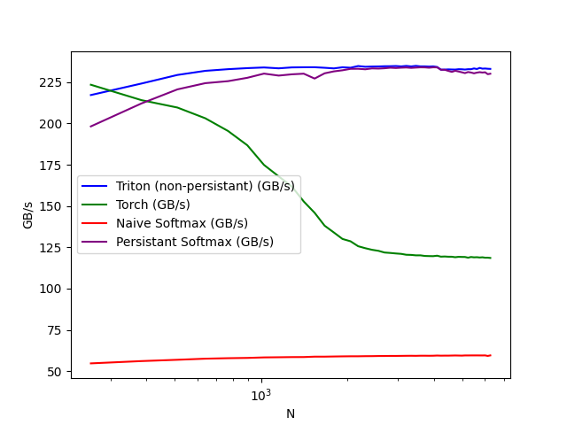
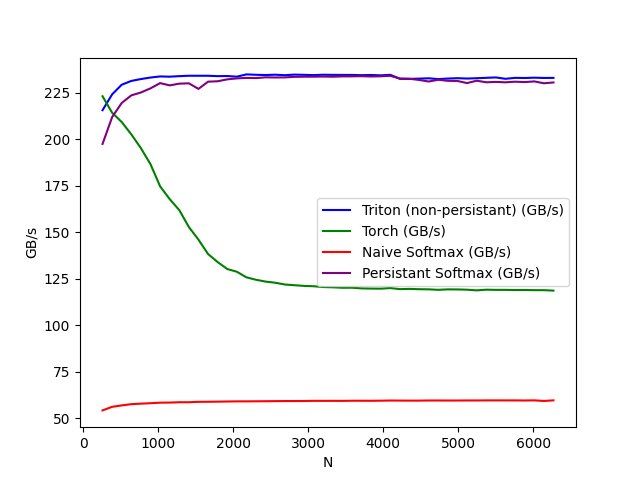
The torch.compile cliff is the most striking thing here. It starts at 223 GB/s at N=256 — actually beating non-persistent Triton at that point — then falls off a cliff, hitting ~119 GB/s by N=1024 and staying flat. At N=6272, it’s delivering 51% of what the hand-written kernel achieves, and both are Triton kernels under the hood.
The reason is that fixed R0_BLOCK=256. When N grows past 256 columns, Inductor can’t fit the whole row in one reduction block and has to fall back to a multi-wave strategy. The hand-written kernel gets around this entirely by setting BLOCK_SIZE = next_power_of_2(n_cols) — each new shape gets a fresh compilation with the right block size.
Persistent softmax starts below non-persistent at small N (197 vs 215 GB/s) because the occupancy calculation and loop overhead don’t pay off when there are already 4096 rows saturating the GPU. By N=2048 both Triton variants are neck and neck at ~233 GB/s.
Naive sits flat at 54–60 GB/s the whole way — about 4× slower — completely bottlenecked by five kernel launches and repeated HBM reads.
Varying M (rows), N = 4096 fixed
| M | Triton (GB/s) | Torch Compiled (GB/s) | Naive (GB/s) | Persistent (GB/s) |
|---|---|---|---|---|
| 32 | 149.8 | 131.3 | 36.3 | 142.0 |
| 64 | 191.6 | 182.9 | 51.3 | 193.2 |
| 128 | 214.8 | 205.2 | 52.8 | 216.0 |
| 256 | 226.9 | 213.6 | 56.0 | 225.2 |
| 512 | 230.4 | 219.0 | 57.6 | 228.8 |
| 3168 | 234.4 | 224.9 | 59.3 | 234.1 |
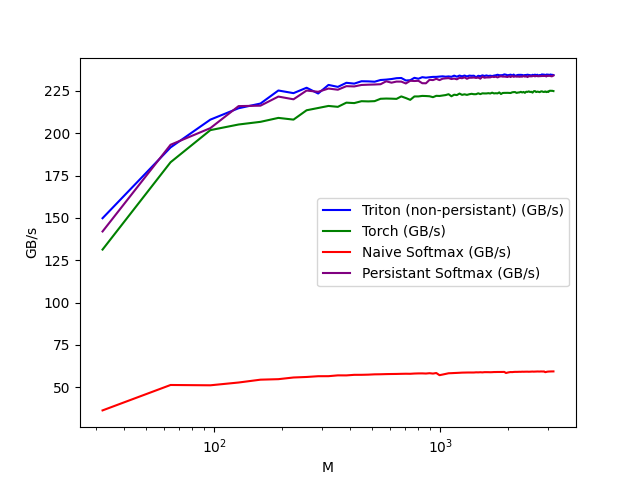
Everything improves as rows increase — more CTAs means better SM saturation. At M=32 all four implementations are well below their peaks simply because the GPU is mostly idle. At M=3168, both Triton variants hit ~234 GB/s while torch compiled settles around 225 GB/s.
The interesting thing at low M is that persistent actually trails non-persistent slightly (142 vs 149 at M=32). With num_programs = min(occupancy * N_SMS, n_rows), at M=32 the clamp kicks in and the persistent kernel degenerates to essentially the same as non-persistent — but with the added overhead of the loop and stage management. That gap closes completely by M=64.
Latency
| M | Triton (ms) | Torch Compiled (ms) | Naive (ms) | Persistent (ms) |
|---|---|---|---|---|
| 32 | 0.0101 | 0.0116 | 0.0433 | 0.0104 |
| 128 | 0.0294 | 0.0307 | 0.1196 | 0.0294 |
| 256 | 0.0554 | 0.0588 | 0.2248 | 0.0558 |
| 512 | 0.1095 | 0.1152 | 0.4374 | 0.1099 |
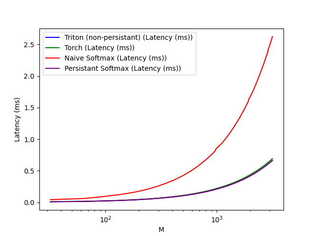
Fused implementations grow linearly with M, as you’d expect for a memory-bound kernel. Triton and torch compiled are within 5% of each other in absolute milliseconds, the gap is mainly in bandwidth efficiency.
Naive softmax’s curve bends upward — super-linear on a log scale. At M=512 it’s already taking 4× longer than any fused kernel. Extrapolate that across 32 transformer layers with multi-head attention and the wall time adds up fast.
What the Persistent Kernel is Actually Doing
The occupancy calculation is the part worth slowing down on:
occupancy = NUM_REGS // (n_regs * num_warps * WARP_SIZE)
occupancy = min(occupancy, SHARED_MEM // size_smem)
num_programs = occupancy * N_SMS
n_regs is read directly from the compiled kernel object after kernel._init_handles(). This is the same number CUDA’s occupancy API would give you, but computed in Python without any manual guessing. The two constraints — register file size and shared memory — are both checked, and whichever is tighter limits occupancy. Launch occupancy × N_SMS CTAs, each running a grid-stride loop, and SMs stay continuously loaded with no wave overhead.
The num_stages=4 in tl.range is what enables the software pipeline. Triton emits instructions to prefetch iteration i+1’s memory while arithmetic for iteration i is still executing, effectively hiding the ~200+ cycle HBM round trip. This shows up as a 1–2 GB/s edge over non-persistent at intermediate row counts.
Both Triton kernels plateau around 234 GB/s regardless of shape. That’s the achievable bandwidth ceiling for this access pattern on this GPU — not the advertised peak, but the real number after memory controller overhead, row-buffer effects, and the read-write mix.
What Didn’t Go as Expected
The torch.compile cliff was steeper than I anticipated. The Triton tutorial frames torch.compile as a strong baseline that custom kernels only marginally beat, so I expected a gradual degradation as N grew. What actually happened was a near-halving of throughput between N=256 and N=1024, then a complete plateau. Once I looked at the generated kernel and saw R0_BLOCK: tl.constexpr = 256 baked in as a compile-time constant, it made sense — but nothing in the tutorial hints that this is the mechanism. I would have expected Inductor to retrace with a larger block when the shape changed. It doesn’t, at least not in this version.
The persistent kernel at small M was a subtler surprise. My prior was that persistent kernels are strictly better — they avoid wave quantization and get L2 reuse, so why wouldn’t they win everywhere? The answer is that at M=32, min(occupancy * N_SMS, n_rows) clamps the grid to 32 CTAs regardless, so you get the loop overhead without any of the benefits. The non-persistent kernel launches the same 32 CTAs but with a simpler dispatch path, and edges it slightly. It’s a small gap (149 vs 142 GB/s) but the direction is counterintuitive until you trace through the math. The persistent design only earns its cost when the row count is large enough to give each SM multiple iterations of work.
Wrapping Up
The takeaway from this isn’t that torch.compile is bad — for most shapes and workloads it’s great. The issue is specifically variable-length reductions. When the compiled kernel specializes on a shape with 256 columns and you then feed it 4096 columns, the blocking strategy it baked in stops working. A hand-written kernel that sets BLOCK_SIZE dynamically doesn’t have this problem because Triton JITs a fresh specialization for each power-of-2 size.
The persistent kernel’s value is less about raw throughput — at saturation it matches non-persistent exactly — and more about correctness of SM utilization across shapes. The occupancy-aware launch pattern is what FlashAttention and similar kernels use under the hood, and it’s worth understanding because it transfers directly to any kernel that loops over a reduction dimension.
The next step from here is online softmax (Milakov & Gimelshein 2018), which fuses the max and sum passes into one, opening the door to fusing softmax with the preceding matmul — which is exactly what FlashAttention does.
| *Code: softmax.py | Compiler output exploration: compile_generated_kernels.py* |